You might remember from the list of sub-modules contained in scipy
that it includes scipy.ndimage which is a useful Image Processing module.
However, scipy tends to focus on only the most basic image processing
algorithms. A younger module, Scikit-Image (skimage) contains some
more recent and more complex image processing functionality.
For real-world applications, a combination of both (and/or additional image processing modules) is often best.
Image Processing: A general overview
While a full introduction to computational image processing is beyond the scope of this workshop, below we include some of the main concepts.
An image is a regular grid of pixel values; a grayscale image will correspond to a 2d array of values and a colour (RGB) image can be represented by a 3d array of values, where the dimension corresponding to colour is of size 3, one per colour channel (sometimes an opacity value is also included as a 4th colour channel, usually denoted “A” for Alpha).
Segmentation
As images are just matrices, most of image processing is concerned with extracting information from these matrices. However, scenes captured in images are often complex meaning that they are composed of background(s), foreground objects, and often several other features. Consequently taking whole-matrix quantities (like mean, median) is rarely sufficient.
Instead, we usually need to segment an image into regions corresponding to foreground, which means objects that we’re interesed in, and background which corresponds to everything else.
Analysis
Once an image has been segmented, further processing might be required (such as splitting touching foreground objects). The final stage in an image processing workflow is to use the segmentation results to extract quantities of interest.
These final segmentations can also form the basis of advanced algorithms such as tracking algorithms if the images are part of a time-series (~film).
Very often, good automated images analysis results can be obtained by chaining relatively simple image processing operations.
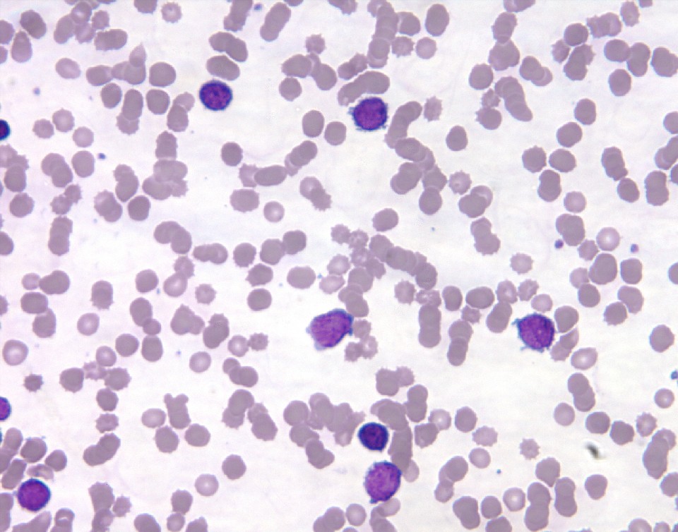
For example, if we were given microscopy images of blood cells with some Leukemic cells, we might want to be able to pick out the Leukemic cells to quantify firstly how many Leukemic cells are present per slide image, and perhaps also quantify other parameters such as their sizes, or circularity.
We can see that by performing just a few “simple” image processing tasks (blurring, automatic threshold detection applied twice), we are able to pick out the Leukemic cells nicely.
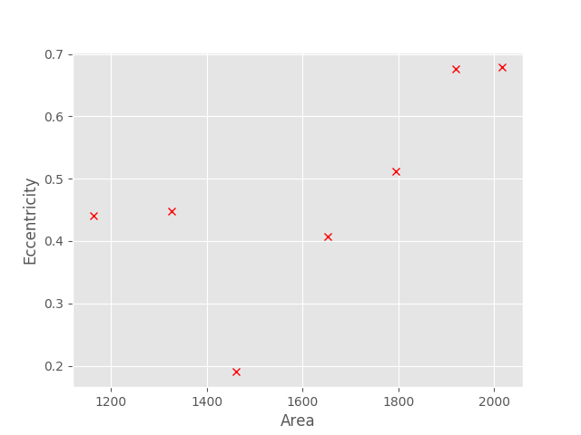
The challenge in quantitative image processing is always in creating these initial segmentation masks. Once the regions have been segmented, the useful data can be harvested and plotted.
For example, from the above images, we could for example plot the area (in pixels) vs the eccentricity (a measure of how non-circular an ellipse is)
To load get started with Scikit-Image, import the submodule
(the core module is called skimage) of interest. For example
to load an image from file, we would use the io submodule;
import skimage.io as skio
skimage.io.imreadim1 = skio.imread("SIMPLE_IMAGE.png")
imstack1 = skio.imread("FILENAME.TIF", plugin="tifffile")
Here I first showed a simple image being read from file using the default
imread function, followed by a second call using the plugin keyword set to
"tifffile", which causes imread to use the tifffile module. This allows
us to handle multi-page (i.e. multi-stack) tiff files.
imread returns a numpy array of either 2 or 3 dimensions, depending on the
file type.
We can then use any normal Numpy operation we wish on the array; e.g.
# Lets output the mean image pixel value
print("The mean of the PNG image is :")
print( im1.mean() )
print("The mean of the TIFF stack (whole stack!) is:")
print( imstack1.mean() )
As we’re dealing with Numpy arrays, we can use Matplotlib’s imshow function to display an image (much as we did during the Matplotlib exercises);
import matplotlib.pyplot as plt
plt.imshow(im1)
plt.show()
Alternatively, the Scikit-Image team have also added image display functions
directly to skimage;
import skimage.viewer as skview
viewer = skview.ImageViewer(im1)
viewer.show()
skimage.viewer is not as full-featured as matplotlib, though new functions
and features are added regularly.
The most basic form of segmentation we can apply is to set a manual threshold. This is akin to using ImageJ’s threshold interface and manually positioning the threshold position.
the_mask = im1 > 100
and that’s it! Thresholding is that simple; as im1 is a Numpy array,
this line will create a boolean array stored in the variable the_mask,
where each element is False if the value of im1 at the corresponding
location was <= 100, or True otherwise.
We can confirm this by viewing our new mask array;
plt.imshow(the_mask)
In fact, we can easily overlay the mask on the original image, by using
the alpha keyword argument to imshow, which sets the transparency of the
image being show;
# Use the `cmap` kwarg to set the colourmap (only works for 2d arrays)
plt.imshow(im1, cmap="gray")
# `the_mask` will be overlaid on `im1` with
# an opacity of 0.4 (maximum 1.0 = fully opaque).
plt.imshow(the_mask, alpha=0.4)
We haven’t really used any image processing functions; let’s remedy that by
automatically determining the threshold value (instead of using a number like
100 that was plucked from thin air!). One of the most common image thresholding
algorithms, which you may know from ImageJ, is the Otsu automatic threshold
determination algorithm.
To use this in skimage, we import the filters submodule;
import skimage.filters as skfilt
thresh_val = skfilt.threshold_otsu(im1)
at this point, thresh_val will hold a single number, which was determined
by the Otsu algorithm to the threshold between what it considered to be
background and foreground pixel intensity values.
We would then generate a mask in the same way as before;
new_mask = im1 > thresh_val
and can continue to perform our next round of image processing operations.
skimage.measure.labelWhile having a binary forefound-background mask is a great first step we are often concerned with multiple objects
In such scenarios, it is usually useful to be able to subsequently determine per-object quantities, where object is often taken to meaning “connected group of foreground pixels”.
Both scipy.ndimage and skimage.measure include a connected-component
labelling function called label; they work in very similar ways, but
be careful that there are subtle differences between.
Basically though, they both work to assign unique labels to each group of
connected foreground pixels (i.e. connected regions of 1s in the mask array).
object_labels = skmeas.label(new_mask)
Now that we know how to get foreground masks that correspond to individual objects, let’s start extracting some useful quantities.
As performing these kinds of information extractions is such a
common task, skimage.measure contains a convenience function
called regionprops (which has the same name as the Matlab equivalent
function in Matlab’s add-on Image Processing toolbox).
regionprops generates a list of RegionPropery objects (collections of
properties), which we can then examine. For example
some_props = skmeas.regionprops(object_labels)

# e.g. let's see the area for the first object
print( some_props[0].area )
We can also collect specific properties (for plotting, e.g.), by using a list comprehension (or a for loop);
areas = [p.area for p in some_props]
Now that we’ve covered some of the core image processing techniques, let’s put them into practice by reproducing the results in the video at the top of the page.
Download the image file:
NOTE
This data was saved as JPG which is a compressed image format that uses lossy compression; but remember -
KEEP YOUR RAW DATA IN UNCOMPRESSED FORMAT.
(or lossless compression such as PNG where appropriate).
Tips
labelling algorithm…regionprops contains both area and eccentricity values for
each region.If the property we are interested in is not present in the output of
regionsprops, we can also calculate the propery ourselves.
There are several relatively straight-forward ways of doing this,
namely to use a utility function like scipy.ndimage’s
labeled_comprehension
or alternatively a list comprehension or for loop over the label values.
For example we could get the object areas using
areas= [ (object_labels == l).sum()
         for l in range(1, object_labels.max()+1) ]
or equivalently
areas = []
for l in range(1, object_labels.max() + 1):
    current_obj = object_labels == l
    areas.append( current_obj.sum() )
Download the image file:

Bonus
Often the actual objects represented in our images touch (or appear to), causing them to be labelled by the same label during the connected component analysis.
In these types of scarios, might be able to use an algorithm known as the Watershed transform to split touching objects.
Note however, that this won’t solve all situations with touching objects, and in some situations the objects simply won’t be resolvable, whilst in others a different strategy for splitting object might be needed.
To apply the watershed transform, import the skimage.morphology submodule,
import skimage.morphology as skmorph
import skimage.feature as skfeature
import scipy.ndimage as ndi

# First generate a distance transformed image
dist = ndi.distance_transform_edt(im1)

# Next generate "markers": regions we are sure belong to different objects
local_maxi = skfeature.peak_local_max(
    dist, indices=False, footprint=np.ones((3, 3)),
    labels=new_mask)
markers = ndi.label(local_maxi)[0]

# Lastly call the watershed transform - it takes the distance transform
# and the markers as inputs (plus optionally the new_mask to delineate objects
# from background)
new_labels = skmorph.watershed(-dist, markers, mask=new_mask)
Image processing techniques are specific to the task being tackled; the previous exercise, while possibly being of interest to some of you, will by no means be useful to all.
Instead of working on additional contrived exercises, please now try and perform image processing that is useful to you using your own data (or find similar data online).