Scipy : Additional scientific computing modules

Numpy is one of the core modules of the Scipy “ecosystem”; however, additional numerical routines are packages in the separate scipy module.

The sub-modules contained in scipy include:

• scipy.cluster : Clustering and cluster analysis
• scipy.fftpack : Fast fourier transform functions
• scipy.integrate : Integration and ODE (Ordinary Differential Equations)
• scipy.interpolate : Numerical interpolation including splines and radial basis function interpolation
• scipy.io : Input/Output functions for e.g. Matlab (.mat) files, wav (sound) files, and netcdf.
• scipy.linalg : Linear algebra functions like eigenvalue analysis, decompositoins, and matrix equation solvers
• scipy.ndimage : Image processing functions (works on high dimensional images - hence nd!)
• scipy.optimize : Optimization (minimize, maximize a function wrt variables), curve fitting, and root finding
• scipy.signal : Signal processing (1d) including convolution, filtering and filter design, and spectral analysis
• scipy.sparse : Sparse matrix support (2d)
• scipy.spatial : Spatial analysis related functions
• scipy.statistical : Statistical analysis including continuous and discreet distributions and a slew of statistical functions

While we don’t have time to cover all of these submodules in detail, we will give a introduction to their general usage with a couple of exercise and then a sample project using a few of them to perform some 1d signal processing.

Exercise : Curve fitting

Curve fitting represents a relatively common research task, and fortunatley Python includes some great curve fitting functionalities.

Some of the more advanced ones are present in additional Scikit libraries, but Scipy includes some of the most common algorithms in the optimize submodule, as well as the odr submodule, which covers the more elaborate “orthogonal distance regression” (as opposed to ordinary least squares used in curve_fit and leastsq).

Load the data contained in the following file

curve_fitting_data_simple

and use the scipy.optimize.curve_fit or scipy.optimize.leastsq (least-squares) fitting function (curve_fit calls leastsq but doesn’t give as much output!) to generate a line of best fit for the data. You shold evaluate several possible functions for the fit including

• A straight line f(x,a,b) = a*x + b
• A quadratic fit f(x,a,b,c) = a*x^2 + b*x + c
• An exponential fit f(x,a,b,c) = a*e^(b*x) + c

Generate an estimate of the goodness of fit to discriminate between these possible models.

Bonus section

Try the same again with the following data (you should be able to just change the filename!)

curve_fitting_data_noisy

You should find that the goodness of fit has become worse. In fact the algorithm used by Scipy’s optimize submodule is not always able to determine which of the models fits best.

Try using the scipy.odr submodule instead; a guide for how to do this can be found here

import numpy as np
import scipy.optimize as scopt
def perform_fitting(filename):
    funcs = {
        'linear'        : lambda x,a,b,c : a*x + b,
        'quadratic'     : lambda x,a,b,c : a*x*x + b*x + c,
        'exponential'   : lambda x,a,b,c : a*np.exp(b*x) + c,
    }

    data = np.fromfile(filename)
    Npoints = len(data)

    taxis = np.arange(Npoints)
    for fname in funcs:

        popt, pcov = scopt.curve_fit( funcs[fname], taxis, data)
        yexact = funcs[fname](taxis, *popt)
        residuals = data - yexact
        ss_err = (residuals**2).sum()
        ss_tot = ((data-data.mean())**2).sum()
        rsquared = 1-(ss_err/ss_tot)

        print("\n\n\nFitting: %s"%fname)
        print("\nCurve fit")
        print("popt:", popt)
        print("pcov:", pcov)
        print("rsquared:", rsquared)

if __name__ == "__main__":
    perform_fitting("curve_fitting_data_simple.txt")

Fitting: quadratic

Curve fit
popt: [  0.27742012   0.43227489  24.42625192]
pcov: [[  1.24062405e-04  -2.35718583e-03   7.07155749e-03]
 [ -2.35718583e-03   4.80617819e-02  -1.65474460e-01]
 [  7.07155749e-03  -1.65474460e-01   8.07571966e-01]]
rsquared: 0.99839145357

Fitting: linear

Curve fit
popt: [ 5.70325725  8.61330482  1.        ]
pcov: inf
rsquared: 0.939693857665

Fitting: exponential

Curve fit
popt: [ 19.98312703   0.10003282   2.07108578]
pcov: [[  2.35952209e-03  -5.30270860e-06  -3.10538435e-03]
 [ -5.30270860e-06   1.20524441e-08   6.87521073e-06]
 [ -3.10538435e-03   6.87521073e-06   4.24287754e-03]]
rsquared: 0.999998872202

Fitting: quadratic

Curve fit
popt: [  0.36402064   1.39338512  33.74952291]
pcov: [[  1.16491630e-02  -2.21334100e-01   6.64002296e-01]
 [ -2.21334100e-01   4.51288594e+00  -1.55376545e+01]
 [  6.64002296e-01  -1.55376545e+01   7.58290698e+01]]
rsquared: 0.932781903212

Fitting: linear

Curve fit
popt: [  8.30977729  13.0003464    1.        ]
pcov: inf
rsquared: 0.887804486031

Fitting: exponential

Curve fit
popt: [ 37.66928574   0.08831645  -6.97576507]
pcov: [[  5.63753689e+02  -6.41775284e-01  -6.99939382e+02]
 [ -6.41775284e-01   7.38443618e-04   7.87263594e-01]
 [ -6.99939382e+02   7.87263594e-01   8.90820497e+02]]
rsquared: 0.933020625779

import scipy.odr as scodr

...
        print("\nODRPACK VERSION")
        funcnow = lambda params, x: funcs[fname](x, *params)
        mod = scodr.Model(funcnow)
        dat = scodr.Data(taxis,data)
        odr = scodr.ODR(dat, mod, beta0 = [1.0, 1.0, 0.0])
        out = odr.run()
        out.pprint()        

Fitting: quadratic

...

ODRPACK VERSION
Beta: [  0.55201606  -0.63943926  31.30145991]
Beta Std Error: [ 0.08980006  1.10407977  1.93744129]
Beta Covariance: [[ 0.00241881 -0.0263813   0.01923865]
 [-0.0263813   0.36563691 -0.35584366]
 [ 0.01923865 -0.35584366  1.12591663]]
Residual Variance: 3.333886943328627
Inverse Condition #: 0.0020568238964839263
Reason(s) for Halting:
  Iteration limit reached

Fitting: linear

...

ODRPACK VERSION
Beta: [ 9.34657515  3.1507637   0.        ]
Beta Std Error: [ 0.78204438  8.56164287  0.        ]
Beta Covariance: [[  0.14923625  -1.41774486   0.        ]
 [ -1.41774486  17.8865157    0.        ]
 [  0.           0.           0.        ]]
Residual Variance: 4.098155829657788
Inverse Condition #: 0.0437541938307872
Reason(s) for Halting:
  Problem is not full rank at solution
  Sum of squares convergence

Fitting: exponential

...

ODRPACK VERSION
Beta: [ 43.9540789    0.08427052 -17.18528396]
Beta Std Error: [  2.68421883e+01   2.80794795e-02   3.04612945e+01]
Beta Covariance: [[  2.69641542e+02  -2.79919119e-01  -3.04410441e+02]
 [ -2.79919119e-01   2.95072729e-04   3.13666736e-01]
 [ -3.04410441e+02   3.13666736e-01   3.47254336e+02]]
Residual Variance: 2.672077403678681
Inverse Condition #: 8.544672221858744e-06
Reason(s) for Halting:
  Sum of squares convergence

Exercise : Interpolating data

Another common use of Scipy is signal interpolation.

Background : Interpolation

Interpolation is often used to resample data, generating data points at a finer spacing than the original data.

A simple example of interpolation is image resizing; when a small image is resized to a larger size, the “in-between” pixel values are generated by interpolating their values based on the nearest original pixel values.

Typical interpolation schemes include nearest, linear, and spline interpolation of various degrees. These terms denote the functional form of the interpolating function.

• nearest neighbor interpolation assigns each interpolated value the value of the nearest original value
• linear interpolation assigns each interpolated value the linearly weighted combination of the neighbouring values; e.g. if the value to be interpolated is 9 times closer to original point B than original point A, then the final interpolated value would be 0.1A + 0.9B.
• Spline interpolation approximates the region between the original data points as quadratic or cubic splines (depending on which spline interpolation order) was selected.

Download the data from here:

data_interpolation

and use “linear” interpolation to interpolate the data to increase so that the new “x axis” has five times as many points between then original limits (i.e. you’ll resample the data to 5 times the density).

Bonus

Run the interpolation with “quadratic” and “cubic” interpolation also (it helps if your interpolation code was in a function!), and you should see much better results!

import scipy.interpolate as scint
import numpy as np
import matplotlib.pyplot as plt     # For plotting



def interp_data(data, kind="quadratic"):
    plt.plot(data[0], data[1])

    func = scint.interp1d(data[0], data[1], kind=kind)

    xnew = np.linspace(data[0][0], data[0][-1], num=5*len(data[0]))
    ynew = func(xnew)

    plt.plot(xnew, ynew, '-r')
    plt.title("Using %s interpolation"%kind)
    plt.show()


if __name__ == '__main__':

    data= np.load("data_interpolation.npy")
    for kind in ["linear", "quadratic", "cubic"]:
        interp_data(data, kind=kind)

Guided exercise: Signal analysis

As you may not have a background in signal processing, as our last exercise, we’ll you through the process instead of leaving you to generate the code from scratch.

Download the wav file (uncompressed audio) from here Wav File.

This sound file will be the basis of our experimentation with some of the additional Scipy modules

Loading data : scipy.io

scipy.io contains file reading functionality to load Matlab .mat files, NetCDF, and wav audio files, amongst others.

We will use the wavfile submodule to load our audio file;

import scipy.io.wavfile as scwav
data, rate = scwav.read("audio_sample.wav")

Next we can inspect the the loaded data using a plot (plotting just the first 500 values),

import matplotlib.pyplot as plt
# Create a "time" axis array; at present there are
# `rate` data-points per second, as rate corresponds to the
# data sample rate.
Nsamples = len(data)
time_axis = np.arange(Nsamples)/rate
plt.plot( time_axis[:500], data[:500])
plt.show()

We should see an audio trace that looks something like

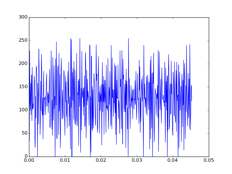
If you have headphones with you and play the audio, you’ll hear a noisy, but still recongnizable sound-bite.

Let’s see if we can improve the sound quality by performing some basic signal processing!

Cleaning the data using : scipy.signal

There are a host of available 1d filters available in Scipy. We’re going to construct a simple low-pass filter using the firwin function;

import scipy.signal as scsig

# Calculate the Nqyist rate
nyq_rate = rate / 2.
# Set a low cutoff frequency of the filter: 1KHz
cutoff_hz = 1000.0
# Length of the filter (number of coefficients, i.e. the filter order + 1)
numtaps = 29
# Use firwin to create a lowpass FIR filter
fir_coeff = scsig.firwin(numtaps, cutoff_hz/nyq_rate)

# Use lfilter to filter the signal with the FIR filter
filtered = scsig.lfilter(fir_coeff, 1.0, data)

# Write the filtered version into an audio file so we can see
# if we can hear a difference!
scwav.write("filtered.wav", rate, filtered)

While “manual” verification by listening to the filtered signal can be useful, we would probably want to also analyze both the original signal and the effect the filtering has had.

Spectral analysis : scipy.fftpack and scipy.signal

To analyze a 1d filter, we often generate a periodogram, which essentially gives us information about the frequency content of the signal. The perriodogram itself is a power-spectrum representation of the Fourier transform of the signal; however, this is not a detailed course in 1d signal processing, so if you have no idea what that means then don’t worry about it!

For sound signals, the periodogram relates directly to the pitches of the sounds in the signal.

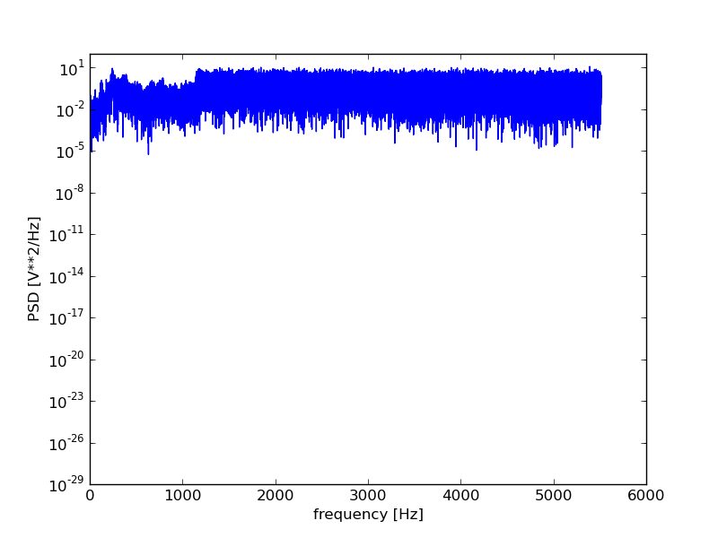
Let’s generate and plot a periodogram using scipy:

plt.figure()
f, Pxx = scsig.periodogram(data.astype(float), rate)
plt.semilogy(f, Pxx)
plt.xlabel('frequency [Hz]')
plt.ylabel('PSD [V**2/Hz]')
plt.show()
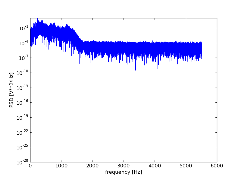
plt.figure()
f, Pxx = scsig.periodogram(filtered.astype(float), rate)
plt.semilogy(f, Pxx)
plt.xlabel('frequency [Hz]')
plt.ylabel('PSD [V**2/Hz]')
plt.show()

For those wanting more control over the spectral analysis, the fftpack submodule offers access to a range of Fast-Fourier transform related functions.

Performing the spectral analysis shows us that the signal did indeed contain a high frequency noise component that the filtering should, at least to some degree have helped remove.

Additional exercise resources

If you would like to further practice Scipy and it’s submodules, please visit this resource.