Now that we’ve loaded some sample data and looked at it a bit, let’s take a step back and think about what that image is.
If we were to use a thermometer to measure the temperature of a solution, or an electrode attached to a ammeter to measure a time-varying current, (such as for a patch-clamp experiment), we know that these measured quantities need to be recorded appropriately and subsequently analysed.
However, when dealing with images, our scientific approach is sometimes forgotten, and we treat images differently, not being careful about data format issues like bit-depth or lossless compression.
When it comes to “analysing” images, this is often left to “by-eye” classification, counting, etc.
While it’s true that our eyes and visual systems are fantastic at pattern recognition and classification, to the extent that in many cases they’re used as the ground-truth when evaluating image processing pipelines, unfortunately they’re not very good scientifically speaking.
This stems mainly from the fact that human perception is subjective, differing both between people and also between the same person at different times.
In addition, we’re not able to be very accurate when quantifying things by eye, such as brightness, size etc.
Before we move onto the more systematic and objective ways that computational image processing techniques (via in this case ImageJ) lets us analyse images, let us quickly recap what an image is.
Most modern optical imaging aparatus consists of two main components; some form of focussing setup (e.g. lenses and mirrors), and the final detector that converts the optical signal (photons) into an electrical signal which will be stored.
The optical components and focussing stage determines for the most part the scale of the scene being imaged, and ranges from very large far away structures (telescope), through to medium to close range, everyday size objects (standard cameras), and finally down to resolving sub-cellular structures or even individual proteins (optical microscopes).
Once the optical signal has traversed the optical setup it is registered.
When these systems were first invented, the only available registration medium
was the eye (followed by drawing what was seen).
Since then, photographic film has long been the standard for capturing images, until
relatively recently, when digital image recording devices were introduced.
Conceptually, these consist of a grid of individual detection units (currently
CMOS and CCD are the most common types of sensor arrays).
Each detection unit converts the intensity of light into an electrical signal
and the whole array of these signals is then encoded into an image format for
storage.
There are many other types of setups which also produce images but don’t use light (photons), such as scanning electron microscopes, atomic force microscopes, ultrasound scanners to name a few. The image processing techniques available through ImageJ work equally well on these types of images also.
For many of these set-ups the images will consist of a grid of pixels.
The grid has a width and height, which we will denote W and H, such that
the grid can be represented by a WxH matrix/array.
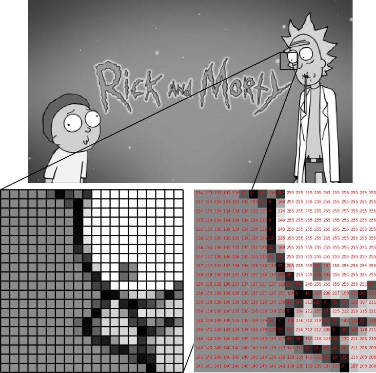
TIP: Pixel inspection tool
ImageJ comes with a “Pixel Inspector” plugin accessible via the toolbar:
- Click the
>>symbol- Select “Pixel inspector”
- Click and drag mouse over image to inspect pixel values.
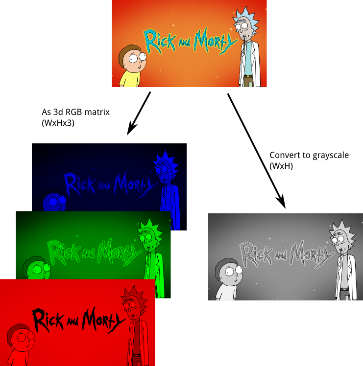
Most images that we’re used to from everyday life are in the form of colour images.
Usually this is stored using RGB (Red-Green-Blue) colour-space, which means that at each location in the image, three values are needed - the amount of red, the amount of blue, and the amount of green.
In this case, the image can be represented as having 3 dimensions, and being of size
W x H x 3.
If we convert the colour image to grayscale, we combine the RGB channel information into a
single quantity (usually a weighted sum of the R, G, and B channels).
This produces a single amount of gray at
each location, and the image matrix returns to being two dimensional.
Now we’ve covered how simple images come as grayscale (2d) or colour with where each pixel has 3 colour values, how about the file format that we use to store that imaging data to disk?
You’ll probably be familiar with some of the common image formats such as JPG/JPEG, PNG, and TIFF.
There is however a crucial difference between the way a format like JPG saves data and how PNG saves data. That difference is down to how the compression algorithms work, as both generally use compression to try and reduce the amount of space needed to store the image information.
JPG uses lossy compression, while PNG uses lossless compression.
Put another way, if pixels were documents, then essentially PNG is similar to a standard ZIP archive, while JPG is like an aggressive archive format which decides which documents are worth keeping, and throws away the rest!
You may have found that JPG files are generally smaller than PNG - now you know why. The “loss of pixels” corresponds to the “compression artifacts” that you may have noticed (especially on more heavily compressesed JPGs) which often look block-like.
TIFF, and in particular, OME-TIFFs are a feature-rich format that allow saving multiple stacks, as well as a wealth of meta-data with your image data. Note however that TIFF does allow for JPG compression, so make sure you never select this when saving data as TIFFs. Also, as OME-TIFF is relatively new, it’s not very widely supported.
PNG on the other hand is a relatively simple format that supports upto 16 bits per channel and upto 4 channels (RGB which we talked about above, and an “alpha” channel which holds transparency information, aka RGBA). There are many additional, proprietary formats - such as Zeiss ZVI, and Leica’s LSM formats.
I would generally recommend avoiding proprietary formats / converting to a more open format such as TIFF (or PNG if appropriate).
The bitdepth or bits-per-pixel (bpp) of an image format refers to the number of bits that are used to store each pixel value. The lowest common bit-depth is 8 bpp, which means that 8 bits are used to store each pixel value. As it is only possible to store 256 (2^8) distinct values with 8 bits, such images usually range between 0 and 255 and will only contain integers.
Scientific data often comes with the option to save at higher bit-depths
(usually up to 16 or 32 in some cases)
which allows for 65536 values to be stored (2^16) - providing a much wider
range of intensities, and therefore detail. Be aware that storing
grayscale data using an 24-bit RGBA format actually only
stores 8 bits per channel - the colour channels will all simply be replicating the same data!
Now that we’ve had a quick introduction to what an image is, and available image formats, let’s get started with ImageJ!