We performed simple thresholding operations in the last section, which involved manually selecting a value at which to separate objects from background.
Less subjective, automated methods for background estimation, or segmentation, also exist.
These include
Threshold)They each have strengths and weaknesses, which depend on the underlying assumptions made.
For example, I routinely use a technique called Median Absolute Deviation (MAD) to estimate the background noise level and variance, and select as signal anything that is ~ 3 variances greater than the background level as it has a very clear assumption about the background level (namely that it is normally distributed noise).
I recommend that you experiment with the various segmentation techniques to find the one that best suits your application.
Repeat the thresholding from exercise 1.3, but experiment with the various automatic thresholding techniques instead of manually selecting the level.
We saw in the simple thresholding that bright areas that touch generally get counted as part of the same region. In some cases this is not desirable as for example we could have multiple cells that are close together.
One technique to overcome this clumping is to use what is known as the watershed transform.
A detailed explanation of the watershed transform can be found here and on wikipedia.
While in some instances applying the watershed transform directly can yield good results, in general there is too much noise in an image to get good segmentation this way. Therefore a common approach is to apply a sequence of operations,
ImageJ contains a function which combined steps 2-4, which is calls watershed under
Process > Binary > Watershed
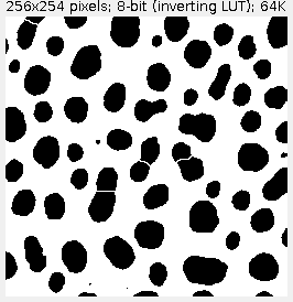
For example, after converting the blobs sample image to binary we have

Then calling watershed gives
Additional details on the distance transform can be found here .
Repeat exercise 1.3, and then perform the same operation, but using the watershed operation before the measurement.
You should notice that there are more objects, some having smaller areas than before. The total area should remain unchanged as we should only have split some touching objects.
To perform watershed and then measure objects in Cell_Colony1.jpg
File > Open ... (or press Ctrl - o)Process > Subtract BackgroundImage > Adjust > Threshold (or press Ctrl - Shift - t)Process > Binary > WatershedAnalyze > Measure (or press Ctrl - m)Scale-space filtering is an advanced filtering technique which enables the extraction of object sizes as well as positions.
The idea is to blur an image at a range of scales, and by combining these scales in the right way 1, one finds that peaks in the resulting nD + 1 (e.g. 2D + 1 = 3D for images) data gives both object positions, x,y,(z..) as well as approximate sizes.
Details
The main operations involved are Gaussian filtering, and taking image derivatives. The motivation for this is that, object peaks correspond to minima in the second derivative, i.e. the change in the curvature, of the smoothed image data.
For example if we were attempting to get positions and sizes of cells, we wouldn’t want to get peaks corresponding to vesicles and other objects that cause the cell image to have small-scale peaks. Therefore we first blur the image over a range of scales such that the minimum scale is smaller than any cell size but larger than any subcellular details, and the maximum scale is larger than any cell size, but smaller than clusters of cells.
This ensures that the peaks in the resulting scale-space representation correspond to cells, and not to subcellular structures or groups of clustered cells.
ImageJ doesn’t contain a scale-space plugin, but the basic operations which allow us to approximate the action of a single scale selection are as follows 2:
Process > Image CalculatorThe resulting image has been scale-space filtered at scale 1.3 x s1.
We’ll find a more useful way of implementing this when we come to macros.
More details about scale-space blob detection can be found here.