2 Data Wrangling
It is estimated that data scientists spend around 50-80% of their time cleaning and manipulating data. This process, known as data wrangling is a key component of modern statistical science, particularly in the age of big data. You should already be familiar with cleaning, manipulating and summarising data using some of R’s core functions. The tidyverse incorporates a suite of packages, such as tidyr and dplyr that are designed to make common data wrangling tasks not only easier to achieve, but also easier to decipher. Readability of the code being a core ideal in the philosophy underpinning the packages.
Great resources are the Data Import Cheat Sheet and Data Transformation Cheat Sheet, which give lots of information about functions available in different
tidyversepackages3.
Before we go any further, if you haven’t already, please load tidyverse:
library(tidyverse)2.1 Tidy data
The architect behind the tidyverse, Hadley Wickham, distinguishes between two types of data set: tidy and messy. This is not to be pejorative towards different ways in which people store and visualise data; rather it is to make a distinction between a specific way of arranging data that is useful to most R analyses, and anything else. In fact Hadley has a neat analogy to a famous Tolstoy quote:
“Tidy datasets are all alike but every messy dataset is messy in its own way.”—Hadley Wickham
Specifically, a tidy data set is one in which:
- rows contain different observations;
- columns contain different variables;
- cells contain values.
The idea of ‘tidy’ data gives rise to the nomenclature of the tidyverse. In this workshop we will see various ways in which datasets can be manipulated to and from the ‘tidy’ format.
2.2 Simple manipulations
Let’s look at a simple example. The iris data set we saw in the last session.
head(iris)## Sepal.Length Sepal.Width Petal.Length Petal.Width Species
## 1 5.1 3.5 1.4 0.2 setosa
## 2 4.9 3.0 1.4 0.2 setosa
## 3 4.7 3.2 1.3 0.2 setosa
## 4 4.6 3.1 1.5 0.2 setosa
## 5 5.0 3.6 1.4 0.2 setosa
## 6 5.4 3.9 1.7 0.4 setosaLet’s start by looking at some basic operations, such as subsetting, sorting and adding new columns. We will compare the tidyverse notation with base R.
2.2.1 Filter rows
One operation we often want to do is to extract a subset of rows according to some criterion. For example, we may want to extract all rows of the iris dataset that correspond to the versicolor species. In base R we can do this as:
iris[iris$Species == "versicolor", ]## Sepal.Length Sepal.Width Petal.Length Petal.Width Species
## 51 7.0 3.2 4.7 1.4 versicolor
## 52 6.4 3.2 4.5 1.5 versicolor
## 53 6.9 3.1 4.9 1.5 versicolor
## 54 5.5 2.3 4.0 1.3 versicolor
## 55 6.5 2.8 4.6 1.5 versicolor
## 56 5.7 2.8 4.5 1.3 versicolorIn tidyverse, we can use a function called filter():
filter(iris, Species == "versicolor")## Sepal.Length Sepal.Width Petal.Length Petal.Width Species
## 1 7.0 3.2 4.7 1.4 versicolor
## 2 6.4 3.2 4.5 1.5 versicolor
## 3 6.9 3.1 4.9 1.5 versicolor
## 4 5.5 2.3 4.0 1.3 versicolor
## 5 6.5 2.8 4.6 1.5 versicolor
## 6 5.7 2.8 4.5 1.3 versicolorNotice some minor differences. The first argument to the filter() function is the data, and the second corresponds to the criteria for filtering. Notice that we did not need to use the $ operator in the filter() function. As with ggplot2 the filter() function knows to look for the column Species in the data set iris.
2.2.2 Sort rows
Another common operation is to sort rows according to some criterion. Let’s say we want to sort rows by Species and then Sepal.Length. In base R we could do this as:
iris[order(iris$Species, iris$Sepal.Length), ]## Sepal.Length Sepal.Width Petal.Length Petal.Width Species
## 14 4.3 3.0 1.1 0.1 setosa
## 9 4.4 2.9 1.4 0.2 setosa
## 39 4.4 3.0 1.3 0.2 setosa
## 43 4.4 3.2 1.3 0.2 setosa
## 42 4.5 2.3 1.3 0.3 setosa
## 4 4.6 3.1 1.5 0.2 setosaIn tidyverse we can use the arrange() function.
arrange(iris, Species, Sepal.Length)## Sepal.Length Sepal.Width Petal.Length Petal.Width Species
## 1 4.3 3.0 1.1 0.1 setosa
## 2 4.4 2.9 1.4 0.2 setosa
## 3 4.4 3.0 1.3 0.2 setosa
## 4 4.4 3.2 1.3 0.2 setosa
## 5 4.5 2.3 1.3 0.3 setosa
## 6 4.6 3.1 1.5 0.2 setosaNotice once again that the first argument to arrange() is the data set, and then subsequent arguments are the columns that we wish to order by. Again, we do not require the $ operator here.
2.2.3 Select columns
Now let’s say that we wish to select just the Species, Sepal.Length and Sepal.Width columns from the data set. There are various ways that we could do this in base R. Here are a few options:
## option 1
iris[, match(c("Species", "Sepal.Length", "Sepal.Width"), colnames(iris))]

## option 2
cbind(Species = iris$Species, Sepal.Length = iris$Sepal.Length,
      Sepal.Width = iris$Sepal.Width)

## option 3 (requires knowing which columns are which)
iris[, c(5, 1, 2)]
In tidyverse we can use the select() function:
select(iris, Species, Sepal.Length, Sepal.Width)## Species Sepal.Length Sepal.Width
## 1 setosa 5.1 3.5
## 2 setosa 4.9 3.0
## 3 setosa 4.7 3.2
## 4 setosa 4.6 3.1
## 5 setosa 5.0 3.6
## 6 setosa 5.4 3.9Notice once again that the first argument to select() is the data set, and then subsequent arguments are the columns that we wish to select; no $ operators required. There is even a set of functions to help extract columns based on pattern matching e.g.
select(iris, Species, starts_with("Sepal"))See the Data Transformation Cheat Sheet for more examples.
Note that we can also remove columns using a - operator e.g.
select(iris, -starts_with("Petal"))or
select(iris, -Petal.Length, -Petal.Width)would remove the petal columns.
2.2.4 Adding columns
Finally, let’s add a new column called Sepal.Length2 that contains the square of the sepal length. In base R:
iris$Sepal.Length2 <- iris$Sepal.Length^2In tidyverse:
mutate(iris, Sepal.Length2 = Sepal.Length^2)## Sepal.Length Sepal.Width Petal.Length Petal.Width Species Sepal.Length2
## 1 5.1 3.5 1.4 0.2 setosa 26.01
## 2 4.9 3.0 1.4 0.2 setosa 24.01
## 3 4.7 3.2 1.3 0.2 setosa 22.09
## 4 4.6 3.1 1.5 0.2 setosa 21.16
## 5 5.0 3.6 1.4 0.2 setosa 25.00
## 6 5.4 3.9 1.7 0.4 setosa 29.16Once again (you should notice a theme here) the first argument to mutate() is the data set, and then the new column as a function of the original column; no $ operators required.
2.2.5 Why bother?
So, why would I choose to use functions such as filter() and mutate() above, when I could have just extracted the correct column of the data, done the appropriate manipulation, and then overwrote or added a new column? There are various reasons:
- These functions are all written in a consistent way. That is, they all take a
data.frameortibbleobject as their initial argument, and they all return a reviseddata.frameortibbleobject. - Their names are informative. In fact they are verbs, corresponding to us doing something specific to our data. This makes the code much more readable, as we will see subsequently.
- They do not require lots of extraneous operators: such as
$operators to extract columns, or quotations around column names. - Functions adhering to these criteria can be developed and expanded to perform all sorts of other operations, such as summarising data over groups.
Note: Some R users like to use a function called
attach. For example,attach(iris)would load the names of the variables in theirisdata frame into the search path in R. This means that you don’t have to use the$command to extract a column. The advantage of this is that the code can often be made clearer e.g.attach(iris) Sepal.Length2 <- Sepal.Length^2The variable names can be removed from the search path by using
detach(iris).However, it is very easy to make errors when using this method, particularly if one wishes to change elements of the underlying data frame. As such I would recommend never using
attach(). For example, the code above does not produce a new column iniriscalledSepal.Length2…
One final and key advantage to the tidyverse paradigm, is that we can use pipes to make our code more succinct.
2.2.6 Pipes (%>%)
Aside: piping comes from Unix scripting, and simply means a chain of commands, such that the results from each command feed into the next one.
Recently, the magrittr package, and subsequently tidyverse have introduced the pipe operator %>% that enables us to chain functions together. Let’s look at an example:
iris %>% filter(Species == "versicolor")## Sepal.Length Sepal.Width Petal.Length Petal.Width Species
## 1 7.0 3.2 4.7 1.4 versicolor
## 2 6.4 3.2 4.5 1.5 versicolor
## 3 6.9 3.1 4.9 1.5 versicolor
## 4 5.5 2.3 4.0 1.3 versicolor
## 5 6.5 2.8 4.6 1.5 versicolor
## 6 5.7 2.8 4.5 1.3 versicolorNotice: when we did this before we would write something like
filter(iris, Species == "versicolor")i.e. we required the first argument offilter()to be adata.frame(ortibble). The pipe operator%>%does this automatically, so the outcome from the left-hand side of the operator is passed as the first argument to the right-hand side function. This makes the code more succinct, and easier to read (because we are not repeating pieces of code).
Pipes can be chained together multiple times. For example:
iris %>%
    filter(Species == "versicolor") %>%
    select(Species, starts_with("Sepal")) %>%
    mutate(Sepal.Length2 = Sepal.Length^2) %>%
    arrange(Sepal.Length)
## Species Sepal.Length Sepal.Width Sepal.Length2
## 1 versicolor 4.9 2.4 24.01
## 2 versicolor 5.0 2.0 25.00
## 3 versicolor 5.0 2.3 25.00
## 4 versicolor 5.1 2.5 26.01
## 5 versicolor 5.2 2.7 27.04
## 6 versicolor 5.4 3.0 29.16I think this is neat! The code is written in a way that is much easier to understand, with each part of the data wrangling process chained together in an intuitive way (once you know the tidyverse functions of course).
Notice that the pipe operator must be at the end of the line if we wish to split the code over multiple lines.
In essence we can read what we have done in much the same way as if we were reading prose. Firstly we take the iris data, filter to extract just those rows corresponding to versicolor species, select species and sepal measurements, mutate the data frame to contain a new column that is the square of the sepal lengths and finally arrange in order of increasing sepal length.
Try doing the same level of data cleaning in Excel as easily…
Note: we can also pass the result of the right-hand side out using the assignment operator
<-e.g.iris <- iris %>% filter(Species = "versicolor")would overwrite theirisdata to produce a new data set with onlyversicolorentries.
Once we’ve got our head around pipes, we can begin to use some of the other useful functions in tidyverse to do some really useful things.
Final point about pipes: the package
magrittr(on which the pipe is implemented) is more general than for justtidyversefunctions. In fact, one can use the pipe to output any object from the left-hand side to the first argument of a function on the right-hand side of the pipe. This is really useful for using functions such assummary()orhead(), that take data frame arguments. Hence I often use pipes like :iris %>% filter(Species == "versicolor") %>% summary().If you load the
magrittrpackage, then there is much more you can do with these ideas. See here for a useful vignette.
2.3 Grouping and summarising
A common thing we might want to do is to produce summaries of some variable for different subsets of the data. For example, we might want to produce an estimate of the mean of the sepal lengths for each species of iris. The dplyr package provides a function group_by() that allows us to group data, and summarise() that allows us to summarise data.
In this case we can think of what we want to do as “grouping” the data by Species and then averaging the Sepal.Length values within each group. Hence,
iris %>%
    group_by(Species) %>%
    summarise(mn = mean(Sepal.Length))
## # A tibble: 3 x 2
## Species mn
## <fct> <dbl>
## 1 setosa 5.01
## 2 versicolor 5.94
## 3 virginica 6.59The summarise() function (note, this is different to the summary() function), applies a function to a data.frame or subsets of a data.frame. Think of it a bit like the tapply function, but with more consistent notation and more power.
2.4 Reshaping data sets
Another key feature of tidyverse is the power it gives you to reshape data sets. The two key functions are gather() and spread(). The gather() function takes multiple columns, and gathers them into key-value pairs. The spread() function is its converse, it takes two columns (key and value) and spreads these into multiple columns. These ideas are best illustrated by an example.
2.4.1 Example: Gapminder
Let’s pull up some data. You should have access to a .csv file called “indicator gapminder gdp_per_capita_ppp.csv”. This is a digital download of the Gapminder GDP per capita data that can be found in the gapminder package. All the data sets used in the Gapminder project can be downloaded from https://www.gapminder.org/data/.
Download this file and save it into your working directory. Now let’s read in the data using the read_csv() function in tidyverse4
gp_income <- read_csv("indicator gapminder gdp_per_capita_ppp.csv")
gp_income
## # A tibble: 262 x 217
## `GDP per capita` `1800` `1801` `1802` `1803` `1804` `1805` `1806` `1807`
## <chr> <int> <int> <int> <int> <int> <int> <int> <int>
## 1 Abkhazia NA NA NA NA NA NA NA NA
## 2 Afghanistan 603 603 603 603 603 603 603 603
## 3 Akrotiri and Dh… NA NA NA NA NA NA NA NA
## 4 Albania 667 667 668 668 668 668 668 668
## 5 Algeria 716 716 717 718 719 720 721 722
## 6 American Samoa NA NA NA NA NA NA NA NA
## 7 Andorra 1197 1199 1201 1204 1206 1208 1210 1212
## 8 Angola 618 620 623 626 628 631 634 637
## 9 Anguilla NA NA NA NA NA NA NA NA
## 10 Antigua and Bar… 757 757 757 757 757 757 757 758
## # … with 252 more rows, and 208 more variables: `1808` <int>,
## # `1809` <int>, `1810` <int>, `1811` <int>, `1812` <int>, `1813` <int>,
## # `1814` <int>, `1815` <int>, `1816` <int>, `1817` <int>, `1818` <int>,
## # `1819` <int>, `1820` <int>, `1821` <int>, `1822` <int>, `1823` <int>,
## # `1824` <int>, `1825` <int>, `1826` <int>, `1827` <int>, `1828` <int>,
## # `1829` <int>, `1830` <int>, `1831` <int>, `1832` <int>, `1833` <int>,
## # `1834` <int>, `1835` <int>, `1836` <int>, `1837` <int>, `1838` <int>,
## # `1839` <int>, `1840` <int>, `1841` <int>, `1842` <int>, `1843` <int>,
## # `1844` <int>, `1845` <int>, `1846` <int>, `1847` <int>, `1848` <int>,
## # `1849` <int>, `1850` <int>, `1851` <int>, `1852` <int>, `1853` <int>,
## # `1854` <int>, `1855` <int>, `1856` <int>, `1857` <int>, `1858` <int>,
## # `1859` <int>, `1860` <int>, `1861` <int>, `1862` <int>, `1863` <int>,
## # `1864` <int>, `1865` <int>, `1866` <int>, `1867` <int>, `1868` <int>,
## # `1869` <int>, `1870` <int>, `1871` <int>, `1872` <int>, `1873` <int>,
## # `1874` <int>, `1875` <int>, `1876` <int>, `1877` <int>, `1878` <int>,
## # `1879` <int>, `1880` <int>, `1881` <int>, `1882` <int>, `1883` <int>,
## # `1884` <int>, `1885` <int>, `1886` <int>, `1887` <int>, `1888` <int>,
## # `1889` <int>, `1890` <int>, `1891` <int>, `1892` <int>, `1893` <int>,
## # `1894` <int>, `1895` <int>, `1896` <int>, `1897` <int>, `1898` <int>,
## # `1899` <int>, `1900` <int>, `1901` <int>, `1902` <int>, `1903` <int>,
## # `1904` <int>, `1905` <int>, `1906` <int>, `1907` <int>, …Before we go any further, notice that the first column is labelled incorrectly as GDP per capita (this is an artefact from the original data set), so let’s rename the first column using the rename() function:
gp_income <- gp_income %>%
    rename(country = "GDP per capita")
gp_income
## # A tibble: 262 x 217
## country `1800` `1801` `1802` `1803` `1804` `1805` `1806` `1807` `1808`
## <chr> <int> <int> <int> <int> <int> <int> <int> <int> <int>
## 1 Abkhaz… NA NA NA NA NA NA NA NA NA
## 2 Afghan… 603 603 603 603 603 603 603 603 603
## 3 Akroti… NA NA NA NA NA NA NA NA NA
## 4 Albania 667 667 668 668 668 668 668 668 668
## 5 Algeria 716 716 717 718 719 720 721 722 723
## 6 Americ… NA NA NA NA NA NA NA NA NA
## 7 Andorra 1197 1199 1201 1204 1206 1208 1210 1212 1215
## 8 Angola 618 620 623 626 628 631 634 637 640
## 9 Anguil… NA NA NA NA NA NA NA NA NA
## 10 Antigu… 757 757 757 757 757 757 757 758 758
## # … with 252 more rows, and 207 more variables: `1809` <int>,
## # `1810` <int>, `1811` <int>, `1812` <int>, `1813` <int>, `1814` <int>,
## # `1815` <int>, `1816` <int>, `1817` <int>, `1818` <int>, `1819` <int>,
## # `1820` <int>, `1821` <int>, `1822` <int>, `1823` <int>, `1824` <int>,
## # `1825` <int>, `1826` <int>, `1827` <int>, `1828` <int>, `1829` <int>,
## # `1830` <int>, `1831` <int>, `1832` <int>, `1833` <int>, `1834` <int>,
## # `1835` <int>, `1836` <int>, `1837` <int>, `1838` <int>, `1839` <int>,
## # `1840` <int>, `1841` <int>, `1842` <int>, `1843` <int>, `1844` <int>,
## # `1845` <int>, `1846` <int>, `1847` <int>, `1848` <int>, `1849` <int>,
## # `1850` <int>, `1851` <int>, `1852` <int>, `1853` <int>, `1854` <int>,
## # `1855` <int>, `1856` <int>, `1857` <int>, `1858` <int>, `1859` <int>,
## # `1860` <int>, `1861` <int>, `1862` <int>, `1863` <int>, `1864` <int>,
## # `1865` <int>, `1866` <int>, `1867` <int>, `1868` <int>, `1869` <int>,
## # `1870` <int>, `1871` <int>, `1872` <int>, `1873` <int>, `1874` <int>,
## # `1875` <int>, `1876` <int>, `1877` <int>, `1878` <int>, `1879` <int>,
## # `1880` <int>, `1881` <int>, `1882` <int>, `1883` <int>, `1884` <int>,
## # `1885` <int>, `1886` <int>, `1887` <int>, `1888` <int>, `1889` <int>,
## # `1890` <int>, `1891` <int>, `1892` <int>, `1893` <int>, `1894` <int>,
## # `1895` <int>, `1896` <int>, `1897` <int>, `1898` <int>, `1899` <int>,
## # `1900` <int>, `1901` <int>, `1902` <int>, `1903` <int>, `1904` <int>,
## # `1905` <int>, `1906` <int>, `1907` <int>, `1908` <int>, …Note we can also use backticks to enclose names that include spaces (which
read_csv()allows).
Notice that the rename() function takes the same form as other tidyverse functions such as filter() or arrange(). We then overwrite the original data frame to keep our workspace neat.
Note: this is OK here because we have a copy of our raw data saved in an external file. This, combined with the use of scripts, means we have a backup of the original data in case anything goes wrong. Don’t overwrite your original data set!
The next thing we need to do is to collapse the year columns down. Ideally we want a column corresponding to country, a column corresponding to year and a final column corresponding to GDP. We are going to do this by using the gather() function. Note that the arguments to gather() are:
data: this gives the name of the data frame;key: gives the name of the column that will contain the collapsed column names (e.g.1800,1801etc.);value: gives the name of the columns that will contain the values in each of the cells of the collapsed column (e.g. the corresponding GDP values);- the final set of arguments correspond to those columns we wish to collapse. Here we want to collapse everything except
country, which we can do using the-operator.
gp_income <- gp_income %>%
    gather(key = year, value = gdp, -country)
gp_income
## # A tibble: 56,592 x 3
## country year gdp
## <chr> <chr> <int>
## 1 Abkhazia 1800 NA
## 2 Afghanistan 1800 603
## 3 Akrotiri and Dhekelia 1800 NA
## 4 Albania 1800 667
## 5 Algeria 1800 716
## 6 American Samoa 1800 NA
## 7 Andorra 1800 1197
## 8 Angola 1800 618
## 9 Anguilla 1800 NA
## 10 Antigua and Barbuda 1800 757
## # … with 56,582 more rowsGreat! This is almost there now. Notice that R has left the new year column as a character vector, so we want to change that:
gp_income <- gp_income %>%
        mutate(year = as.numeric(year))
Also, there is quite a lot of extraneous information in the data. Firstly, there were some mostly empty rows in Excel, which manifest as missing values when the data were read into R:
sum(is.na(gp_income$country))## [1] 432We can examine these rows by filtering.
gp_income %>% filter(is.na(country)) %>% summary()## country year gdp
## Length:432 Min. :1800 Min. :36327
## Class :character 1st Qu.:1854 1st Qu.:36327
## Mode :character Median :1908 Median :36327
## Mean :1908 Mean :36327
## 3rd Qu.:1961 3rd Qu.:36327
## Max. :2015 Max. :36327
## NA's :431We can see from the summary that only one row has any GDP information, and indeed in the original data there was a single additional point that could be found in cell HE263 of the original Excel file. I think this is an artefact of the original data, and as such we will remove it here:
gp_income <- gp_income %>% filter(!is.na(country))We can also remove the rows that have no GDP information if we so wish (which are denoted by missing values—NA):
gp_income <- gp_income %>% filter(!is.na(gdp))Finally, we will restrict ourselves to looking at the data from 1990 onwards:
gp_income <- gp_income %>% filter(year > 1990)
head(gp_income)
## # A tibble: 6 x 3
## country year gdp
## <chr> <dbl> <int>
## 1 Afghanistan 1991 1022
## 2 Albania 1991 3081
## 3 Algeria 1991 9748
## 4 Andorra 1991 28029
## 5 Angola 1991 4056
## 6 Antigua and Barbuda 1991 17361summary(gp_income)## country year gdp
## Length:5075 Min. :1991 Min. : 142
## Class :character 1st Qu.:1997 1st Qu.: 2809
## Mode :character Median :2003 Median : 8476
## Mean :2003 Mean : 15743
## 3rd Qu.:2009 3rd Qu.: 21950
## Max. :2015 Max. :148374Phew! this took some effort, but we’ve managed to end up with a fairly clean data set that we can plot, summarise etc.
To do all of the previous data cleaning operation using pipes, we can write:
gp_income <- read_csv("indicator gapminder gdp_per_capita_ppp.csv") %>%
                rename(country = `GDP per capita`) %>%
                gather(year, gdp, -country) %>%
                mutate(year = as.numeric(year)) %>%
                filter(!is.na(country)) %>%
                filter(!is.na(gdp)) %>%
                filter(year > 1990)
Now we can begin to motor. For example, we might want to produce a mean GDP for each country, averaging over years. In this case we can think of “grouping” the data by country and then averaging the GDP values within each group (as we have seen before):
gp_income %>%
    group_by(country) %>%
    summarise(mn = mean(gdp))
## # A tibble: 203 x 2
## country mn
## <chr> <dbl>
## 1 Afghanistan 1221.
## 2 Albania 6549.
## 3 Algeria 11081.
## 4 Andorra 35455.
## 5 Angola 4888.
## 6 Antigua and Barbuda 20017.
## 7 Argentina 12909.
## 8 Armenia 4626.
## 9 Aruba 38928.
## 10 Australia 36583.
## # … with 193 more rowsWe must be a bit careful here, since we may have less samples for some countries/years than for others. This affects the uncertainty in our estimates, though it is not too difficult to extract standard errors for each grouping and thus produce confidence intervals to quantify which estimates are more uncertain than others (this is where proper statistical modelling is paramount).
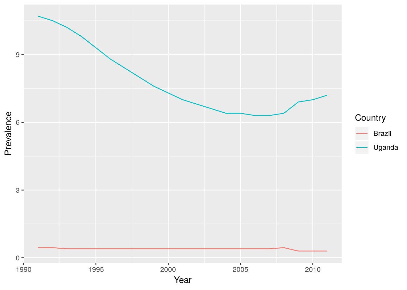
gp_hiv using the tools in tidyverse that we introduced above. The dataset needs to run from 1991 onwards, and we want to end up with columns country, year and prevalence. [Note that a couple of the years have no values in the data set, and by default R reads these columns in as character columns. Hence when you gather() the data to create a prevalence column, all the numbers will be converted into characters. One way to deal with this is to convert the column back into numbers once you have filtered away all the guff!]
ggplot2, and notice that the first argument to the ggplot() function is a data.frame! You might also have to convert the year column to a numeric…]
2.5 Joins
We now have two data sets: gp_income and gp_hiv. In order to visualise and analyse them, we need to link them together. A key skill to have in data manipulation is the ability to join data sets (or tables) together. The dplyr package provides various functions to do this, depending on how you want to join the tables.
In case you haven’t managed to complete the last task, the
gp_hivdata is available as “gp_hiv.rds”. You can read this into R usinggp_hiv <- readRDS("gp_hiv.rds")and continue with the practical.
In order to join two tables, you must have one or more variables in common. In this case we want to match by country and year, to produce a data set that contains country, year, gdp and prevalence.
There should be at most one entry for each country \(\times\) year combination. We can check this using the count() function in dplyr:
gp_income %>% count(country, year) %>% summary()## country year n
## Length:5075 Min. :1991 Min. :1
## Class :character 1st Qu.:1997 1st Qu.:1
## Mode :character Median :2003 Median :1
## Mean :2003 Mean :1
## 3rd Qu.:2009 3rd Qu.:1
## Max. :2015 Max. :1gp_hiv %>% count(country, year) %>% summary()## country year n
## Length:3066 Min. :1991 Min. :1
## Class :character 1st Qu.:1996 1st Qu.:1
## Mode :character Median :2001 Median :1
## Mean :2001 Mean :1
## 3rd Qu.:2006 3rd Qu.:1
## Max. :2011 Max. :1
count()counts the numbers of entries in each combination of the provided variables: in this caseyearandcountry. Thesummary()function is to provide a straightforward way to see that all thecountry\(\times\)yearcombinations have one entry only.
This should make it straightforward to join. Hence,
gp <- inner_join(gp_income, gp_hiv, by = c("year", "country"))
gp
## # A tibble: 3,066 x 4
## country year gdp prevalence
## <chr> <dbl> <int> <dbl>
## 1 Algeria 1991 9748 0.06
## 2 Angola 1991 4056 0.8
## 3 Argentina 1991 9333 0.3
## 4 Armenia 1991 3329 0.06
## 5 Australia 1991 28122 0.1
## 6 Austria 1991 31802 0.06
## 7 Azerbaijan 1991 8323 0.06
## 8 Bahamas 1991 22841 3.8
## 9 Bangladesh 1991 1287 0.06
## 10 Barbados 1991 12573 0.06
## # … with 3,056 more rowsThe inner_join() function takes two data sets, and returns a combined data set with entries that match on both country and year. Any rows from either data set that do not match the other data set are removed. To have a look at entries that differ on the matching criteria between the data sets, then we can use either semi_join() or anti_join() (please see Data Transformation Cheat Sheet). For example, the function anti_join(gp_income, gp_hiv, by = c("year", "country")) will return all rows of gp_income that can’t be matched to gp_hiv, and visa-versa for anti_join(gp_hiv, gp_income, by = c("year", "country")):
anti_join(gp_income, gp_hiv, by = c("year", "country"))## # A tibble: 2,009 x 3
## country year gdp
## <chr> <dbl> <int>
## 1 Afghanistan 1991 1022
## 2 Albania 1991 3081
## 3 Andorra 1991 28029
## 4 Antigua and Barbuda 1991 17361
## 5 Aruba 1991 38310
## 6 Bahrain 1991 38315
## 7 Bermuda 1991 39322
## 8 Bosnia and Herzegovina 1991 2613
## 9 Brunei 1991 77275
## 10 Cape Verde 1991 1597
## # … with 1,999 more rowsanti_join(gp_hiv, gp_income, by = c("year", "country"))## # A tibble: 0 x 3
## # … with 3 variables: country <chr>, year <dbl>, prevalence <dbl>We can see that there are 2009 entries present in gp_income that can’t be matched to gp_hiv, but 0 entries in gp_hiv that can’t be matched to gp_income.
2.5.1 Types of join
Inner joins return only those rows that can be matched in both data sets, it discards any rows from either data frame that can’t be matched.
Outer joins retain rows that don’t match, depending on the type of join. Left outer joins retain rows from the left-hand side that don’t match the right, but discard rows from the right that don’t match the left. Right outer joins retain rows from the right-hand side that don’t match the left, but discard rows from the left that don’t match the right. Full outer joins return all rows that don’t match. R uses missing values (NA) to fill in gaps that it can’t match. For example,
left_join(gp_income, gp_hiv, by = c("year", "country"))## # A tibble: 5,075 x 4
## country year gdp prevalence
## <chr> <dbl> <int> <dbl>
## 1 Afghanistan 1991 1022 NA
## 2 Albania 1991 3081 NA
## 3 Algeria 1991 9748 0.06
## 4 Andorra 1991 28029 NA
## 5 Angola 1991 4056 0.8
## 6 Antigua and Barbuda 1991 17361 NA
## 7 Argentina 1991 9333 0.3
## 8 Armenia 1991 3329 0.06
## 9 Aruba 1991 38310 NA
## 10 Australia 1991 28122 0.1
## # … with 5,065 more rowsHere we can see that there is no prevalence data for Afghanistan in 1991, so R has included the row but with a missing value (NA) in place of the prevalence data. In the inner_join above, this row was removed. Try exploring right- and full- outer joins.
right_join(gp_income, gp_hiv, by = c("year", "country"))## # A tibble: 3,066 x 4
## country year gdp prevalence
## <chr> <dbl> <int> <dbl>
## 1 Algeria 1991 9748 0.06
## 2 Angola 1991 4056 0.8
## 3 Argentina 1991 9333 0.3
## 4 Armenia 1991 3329 0.06
## 5 Australia 1991 28122 0.1
## 6 Austria 1991 31802 0.06
## 7 Azerbaijan 1991 8323 0.06
## 8 Bahamas 1991 22841 3.8
## 9 Bangladesh 1991 1287 0.06
## 10 Barbados 1991 12573 0.06
## # … with 3,056 more rowsfull_join(gp_income, gp_hiv, by = c("year", "country"))## # A tibble: 5,075 x 4
## country year gdp prevalence
## <chr> <dbl> <int> <dbl>
## 1 Afghanistan 1991 1022 NA
## 2 Albania 1991 3081 NA
## 3 Algeria 1991 9748 0.06
## 4 Andorra 1991 28029 NA
## 5 Angola 1991 4056 0.8
## 6 Antigua and Barbuda 1991 17361 NA
## 7 Argentina 1991 9333 0.3
## 8 Armenia 1991 3329 0.06
## 9 Aruba 1991 38310 NA
## 10 Australia 1991 28122 0.1
## # … with 5,065 more rowsWhat do you notice about the left- and full- outer joins here? Why is this so?
There is a great cheat sheet for joining by Jenny Bryan that can be found here.
Hopefully we have now cleaned two data sets, merged them together and can now proceed with visualising them. We want to plot HIV prevalence against GDP per capita, and so an inner join is sufficient here.
ggplot2, produce a plot of HIV prevalence in 15-49 year olds against \(\log_{10}\) (GDP per capita) for 1991, 1997, 2005 and 2011, where each point represents a country.
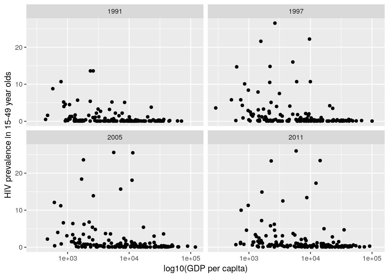
gp data you have already created.
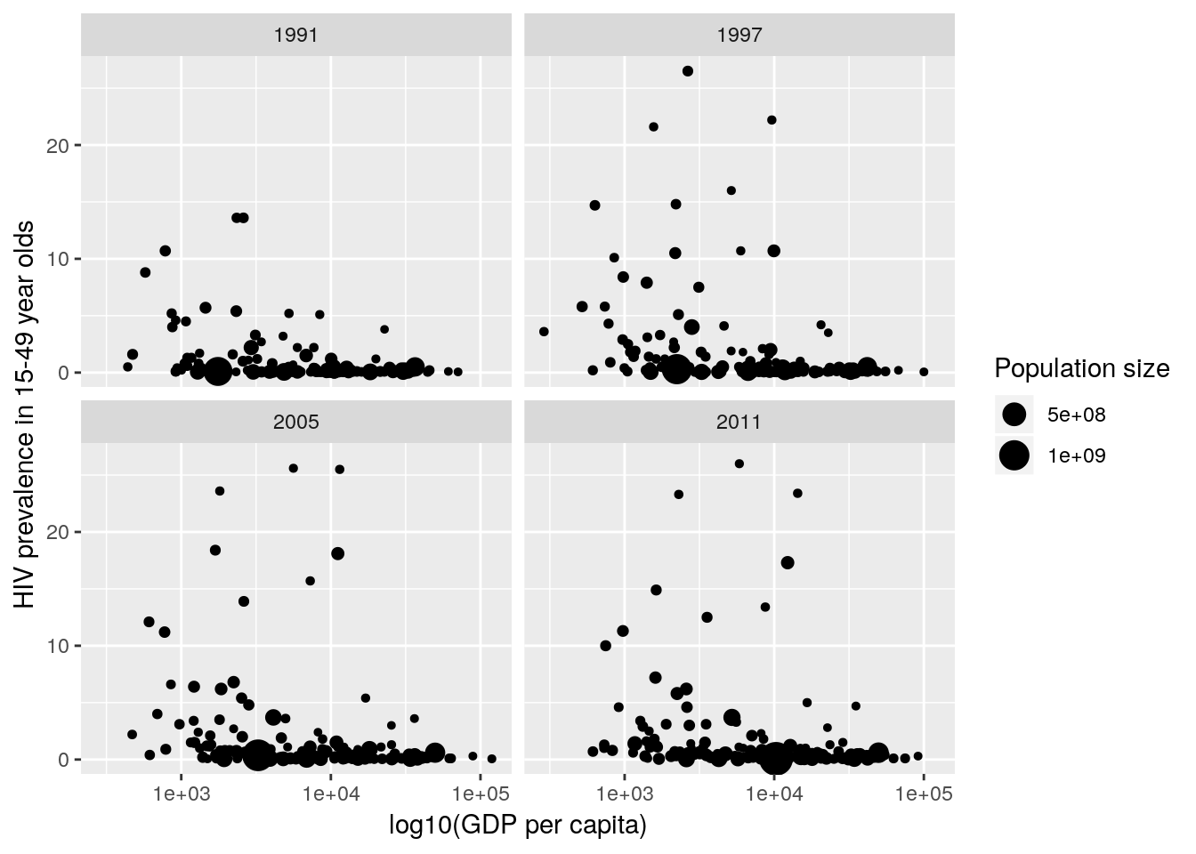
country and where the point sizes are scaled by population size.
2.6 Comprehensive example—Population pyramids
Population pyramids are commonly used by demographers to illustrate age and sex structure of a country’s population. A schematic example of a population pyramid is shown in Figure 2.1.
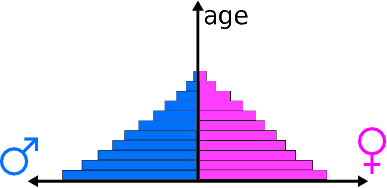
Figure 2.1: Schematic diagram of a population pyramid (source: Wikipedia)
Here we look at the population counts for three countries: Germany, Mexico and the US from the year 2000. You should have access to three files: “Germanypop.csv”, “Mexicopop.csv” and “USpop.csv”, each with the following columns:
- male: Population counts for males (\(\times\) 1000);
- female: Population counts for females (\(\times\) 1000).
Each row corresponds to an age class, in the order: 0–4, 5–9, 10–14, 15–19, 20–24, 25–29, 30–34, 35–39, 40–44, 45–49, 50–54, 55–59, 60–64, 65–69, 70–74 and 75–79. Mexico then has a final age class of 80+; Germany has final age classes of 80–84 and 85+; and the US has final age classes of 80–84, 85–89, 90–94 and 95+.
Original source: US Census
(I downloaded these data sets from the very excellent QELP website: http://www.seattlecentral.edu/qelp/sets/032/032.html, and wish to thank the authors for providing a brilliant resource for teaching statistics.)
In this exercise we will load these data into R, wrangle them into a useful format and then produce a population pyramid using ggplot2. We will aim to do all of this using a tidyverse workflow where possible.
2.6.1 Data Wrangling
Firstly, we read the three data files into R, storing them as tibble objects called germany, mexico and us.
## read German data in
germany <- read_csv("Germanypop.csv")

## read Mexican data in
mexico <- read_csv("Mexicopop.csv")

## read US data in
us <- read_csv("USpop.csv")
We now need to bind these data sets together. One issue is that these three data sets have different age classes. If we want to join the tables together, we need to set consistent groupings in each data set. For this we will set the maximum age class for each country to be "80+". Hence for Mexico we do not need to do anything, but for Germany and the US we will need to group together the latter categories.
Let’s do the US first.
us <- us %>%
    mutate(age = ifelse(age == "80-84", "80+", age)) %>%
    mutate(age = ifelse(age == "85-89", "80+", age)) %>%
    mutate(age = ifelse(age == "90-94", "80+", age)) %>%
    mutate(age = ifelse(age == "95+", "80+", age)) %>%
    group_by(age) %>%
summarise(male = sum(male), female = sum(female))germany.
We will now join the three data sets together on the age column, before gathering together the male and female counts for each country into two columns: one of population counts (pop) and one relating to sex (which actually captures sex and country at this stage). We will then separate the sex and country values into two separate columns. We do this using a single piped workflow that avoids us having to create lots of temporary objects.
pop <- germany %>%
        inner_join(mexico, "age", suffix = c("_Germany", "_Mexico")) %>%
        inner_join(us, "age") %>%
        rename(male_US = male, female_US = female) %>%
        gather("country", "pop", -age) %>%
        separate(country, c("sex", "country"), sep = "_") %>%
        mutate(country = factor(country), sex = factor(sex)) %>%
        mutate(age = factor(age, levels = unique(mexico$age)))
pop
## # A tibble: 102 x 4
## age sex country pop
## <fct> <fct> <fct> <int>
## 1 0-4 male Germany 2055
## 2 10-14 male Germany 2458
## 3 15-19 male Germany 2404
## 4 20-24 male Germany 2361
## 5 25-29 male Germany 2623
## 6 30-34 male Germany 3573
## 7 35-39 male Germany 3756
## 8 40-44 male Germany 3263
## 9 45-49 male Germany 2883
## 10 50-54 male Germany 2432
## # … with 92 more rows2.6.2 Visualisation
Finally, we have wrangled our data into a useful form for data analysis. Now we will try and plot some population pyramids using ggplot2. We do this by tricking ggplot into plotting stacked barplots, with males being plotted below the zero line, and females above the zero line. We then flip the axes and use faceting and colours to denote countries and sex respectively.
ggplot(pop, aes(x = age, y = ifelse(sex == "male", -pop, pop), fill = sex)) +
    geom_bar(stat = "identity") +
    scale_y_continuous(
        breaks = signif(seq(-max(pop$pop), max(pop$pop), length.out = 5), 2),
        labels = abs(signif(seq(-max(pop$pop), max(pop$pop), length.out = 5), 2))
    ) +
    coord_flip() +
    facet_wrap(~ country, ncol = 1) +
    ylab("Population counts (x1000)") +
    xlab("Age (yrs)") +
    labs(fill = "Sex")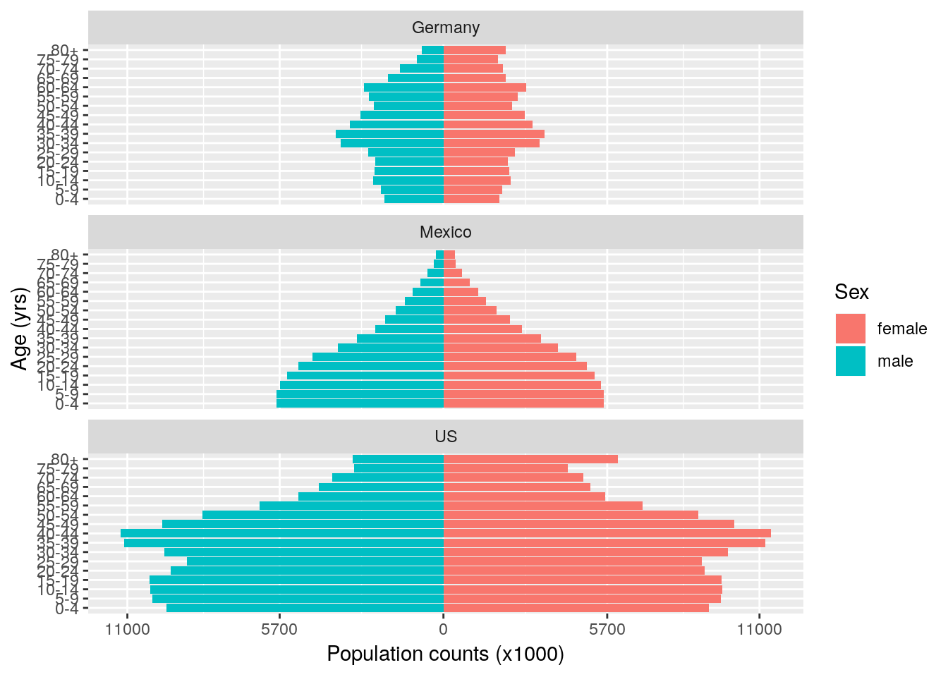
Beautiful isn’t it? (The stereotypical gender colours are purely a coincidence due to the defaults in ggplot2, please feel free to change them to something less egregious.) These plots are hugely informative. We know that countries experiencing fast population growth typically have a large number of individuals of reproductive age, with a wider base to the pyramid. In contrast, populations that have slow, static or even negative growth typically have more older individuals; their pyramids tend to be wider at the top. We can also see that the US has a much larger population than Mexico or Germany.
2.6.3 Summarisation
In the year 2000, the population distribution of Mexico shows a very bottom-heavy pattern, suggesting few older people, but a large number of young and middle-age people. In fact we can quantify this directly as:
pop %>%
    group_by(country, age) %>%
    summarise(pop = sum(pop)) %>%
    arrange(country, age) %>%
    mutate(cumprop = cumsum(pop / sum(pop))) %>%
    select(-pop) %>%
    spread(age, cumprop)
## # A tibble: 3 x 18
## # Groups: country [3]
## country `0-4` `5-9` `10-14` `15-19` `20-24` `25-29` `30-34` `35-39`
## <fct> <dbl> <dbl> <dbl> <dbl> <dbl> <dbl> <dbl> <dbl>
## 1 Germany 0.0483 0.0994 0.157 0.214 0.269 0.331 0.415 0.503
## 2 Mexico 0.114 0.227 0.338 0.445 0.545 0.637 0.713 0.777
## 3 US 0.0685 0.140 0.212 0.285 0.352 0.417 0.488 0.569
## # … with 9 more variables: `40-44` <dbl>, `45-49` <dbl>, `50-54` <dbl>,
## # `55-59` <dbl>, `60-64` <dbl>, `65-69` <dbl>, `70-74` <dbl>,
## # `75-79` <dbl>, `80+` <dbl>spread() function to produce a table that is not in ‘tidy’ format, but is better for visualising these specific outcomes.
We can see here that around 55% of Mexicans are younger than 25, compared to around 27% of Germans and 35% of Americans. We can also look at these figures split by sex:
pop %>%
    arrange(country, sex, age) %>%
    group_by(country, sex) %>%
    mutate(cumprop = cumsum(pop / sum(pop))) %>%
    select(-pop) %>%
    spread(age, cumprop)
## # A tibble: 6 x 19
## # Groups: country, sex [6]
## sex country `0-4` `5-9` `10-14` `15-19` `20-24` `25-29` `30-34`
## <fct> <fct> <dbl> <dbl> <dbl> <dbl> <dbl> <dbl> <dbl>
## 1 fema… Germany 0.0460 0.0946 0.150 0.203 0.257 0.315 0.395
## 2 fema… Mexico 0.110 0.219 0.327 0.430 0.529 0.619 0.698
## 3 fema… US 0.0655 0.134 0.203 0.272 0.336 0.400 0.471
## 4 male Germany 0.0508 0.104 0.165 0.225 0.283 0.348 0.436
## 5 male Mexico 0.118 0.235 0.350 0.460 0.562 0.654 0.729
## 6 male US 0.0715 0.147 0.222 0.298 0.369 0.435 0.507
## # … with 10 more variables: `35-39` <dbl>, `40-44` <dbl>, `45-49` <dbl>,
## # `50-54` <dbl>, `55-59` <dbl>, `60-64` <dbl>, `65-69` <dbl>,
## # `70-74` <dbl>, `75-79` <dbl>, `80+` <dbl>Mexico also has a very high proportion of young females: in fact 33% of the current population of women are of pre-reproductive age (0–14 years) and 49% are of reproductive age (15–44). This means Mexico’s population is expected to rapidly increase in the near future. A general pattern is that as countries transition from more agricultural economies to more industrialised economies, birth rates drop (due to better access to family planning, increased job opportunities for women, and various other factors). As soon as birth rates approach death rates then population growth declines, and the population pyramid becomes more top-heavy. The US is currently classed as a medium-growth country, and Germany a negative-growth country. The population pyramid plot also helps visualise the overall differences in population sizes between the three countries.
A good description of population demographics can be found in this short video:
Another great site on these sorts of topics is the OurWorldInData project.
Note that we do not make distinctions between which functions belong to which
tidyversepackages here. Most of the functions we will use belong to eitherreadr,dplyr,tidyrorggplot2. Information on these packages can be found on the cheat sheets.↩Note that this is different than the
read.csv()function in base R. It doesn’t convertcharactercolumns tofactorcolumns, and returns atibbleby default.↩