4 Raster: Working with raster data
This chapter will introduce you to some of the key concepts surrounding the use of raster spatial data in R. You will learn the basics of how to create, manipulate, import and export raster data.
4.1 Setup
4.2 Importing and plotting raster data
Getting raster data in is easy and can be done using the following commands:
The raster function is used for single layer files and the stack function for
raster datasets with multiple layers, or for combining single layer rasters into
a multilayer raster.
4.2.1 Importing a raster layer
A single raster layer is easily imported. Here we load an example from the system repository:
4.2.2 Importing a raster stack
Rasters can be stacked and this is particularly useful for RGB layers in a raster. For example, we can illustrate this using the R logo:
## [1] 3There are three layers in sRLogo representing the red, green and blue
channels (RGB). These can be plotted individually:
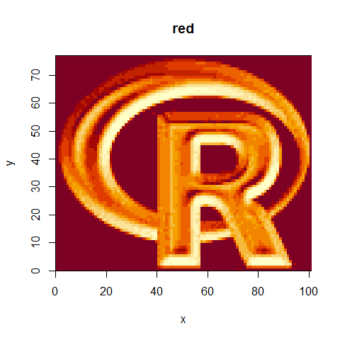
Figure 4.1: The R logo 1

Figure 4.2: The R logo 2
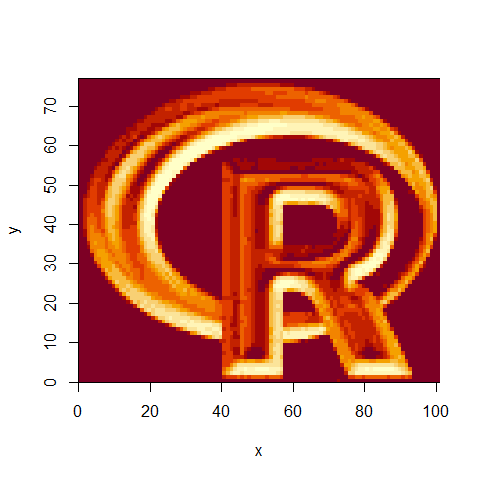
Figure 4.3: The R logo 3
Note that the initial code to call these layers can vary. The first uses
the options within the image function, the second calls the name of the layer
green and finally the last uses the index of the layer. These are useful to
know as it may be appropriate to use different calls for different
purposes - here it makes little difference.
These data may be more useful if plotted as an RGB plot. R isn’t great at this
but for a quick visualisation we can use plotRGB:

Figure 4.4: R Logo with a linear stretch (default)
There are few tricks to plotRGB worth exploring such as changing the stretch:

Figure 4.5: R Logo with a histogram equalised stretch
And changing the order of the bands - useful when RGB are not in the correct order:

Figure 4.6: R Logo with different order of bands
4.2.3 A random synthetic raster
Sometimes it can be useful to generate a random synthetic dataset. This could be for adding random noise to a dataset or for simple testing, or creating a reproducible example:
The success of this can be checked in a number of ways:
Similarly, a synthetic raster stack can be generated by simply manipulating the values:
4.2.4 Rasterising Vector Data
Given that raster data is generally more efficient to work with, and that sometimes vector data is not suitable for a particular analysis, you may wish to rasterise your vector data. This is easily achieved in R, although you must carefully consider how your spatial data will be represented in its new form.
4.2.4.1 Points
For this example, we will create a random set of points:
And some accompanying random values:
The rasterize function can then be utilised to convert from vector to raster format:
rPoints0 <- raster(ncols=36, nrows=18)
rPoints1 <- rasterize(xy, rPoints0)
rPoints2 <- rasterize(xy, rPoints0, field = z)
rPoints3 <- rasterize(xy, rPoints0, field = zzz) # Note the form of the object create (RasterBrick)
plot(rPoints3)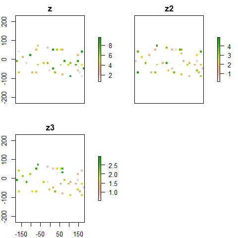
Similarly, rasterize can also be used on spatial objects, such as SpatialPointsDataFrames:
dfPoints <- data.frame(xy, name = zzz)
coordinates(dfPoints) <- ~x+y # Note the change in object type
rPoints4 <- rasterize(dfPoints, rPoints0, zzz)
plot(rPoints4)
4.2.4.2 Lines
For this example, we will create some lines:
cds1 <- rbind(c(-180,-20), c(-140,55), c(10, 0), c(-140,-60))
cds2 <- rbind(c(-10,0), c(140,60), c(160,0), c(140,-55))
cds3 <- rbind(c(-125,0), c(0,60), c(40,5), c(15,-45))
lines <- spLines(cds1, cds2, cds3)
rLines0 <- raster(ncols=90, nrows=45)
rLines1 <- rasterize(lines, rLines0)
plot(rLines1)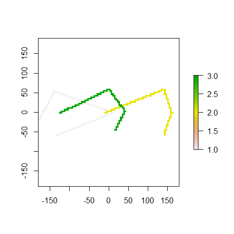
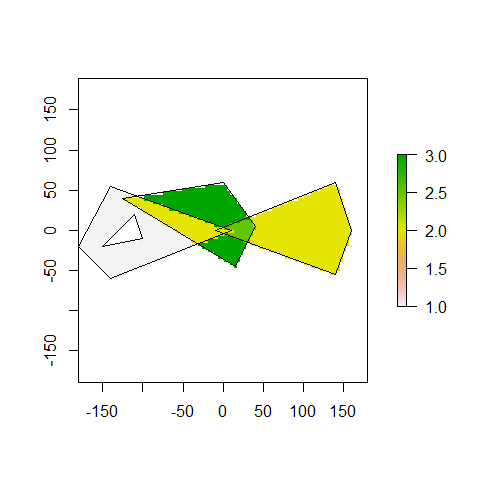
4.2.4.3 Polygons
For this example, we will create some polygons:
p1 <- rbind(c(-180,-20), c(-140,55), c(10, 0), c(-140,-60), c(-180,-20))
hole <- rbind(c(-150,-20), c(-100,-10), c(-110,20), c(-150,-20))
p1 <- list(p1, hole)
p2 <- rbind(c(-10,0), c(140,60), c(160,0), c(140,-55), c(-10,0))
p3 <- rbind(c(-125,40), c(0,60), c(40,5), c(15,-45), c(-125,40))
pols <- spPolygons(p1, p2, p3)
rPols0 <- raster(ncol=90, nrow=45)
rPols1 <- rasterize(pols, rPols0)
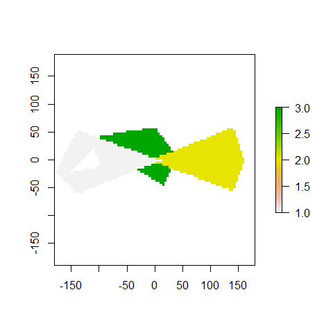
rPols2 <- rasterize(pols, rPols0, fun="min")
rPols3 <- rasterize(pols, rPols0, fun="mean")
plot(rPols1)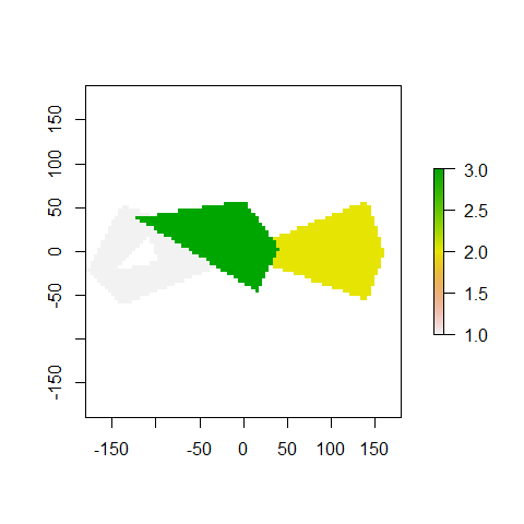
4.3 Real examples
Moving on from creating, plotting and manipulating non-spatial or synthetic raster data, we will now use some real world examples to further explore raster data in R.
4.3.1 Elevation data
Here we use a vector file to define our area of interest when requesting elevation data from an external API:
## OGR data source with driver: ESRI Shapefile
## Source: "C:\Git\spatial_data_analysis\data\ukdata\england_ct_2001.shp", layer: "england_ct_2001"
## with 18 features
## It has 2 fieldsThe elevation data is accessed using the elevatr package. more details can be found here
## Merging DEMs## Reprojecting DEM to original projection## Note: Elevation units are in meters.
## Note: The coordinate reference system is:
## +proj=longlat +datum=WGS84 +ellps=WGS84 +towgs84=0,0,0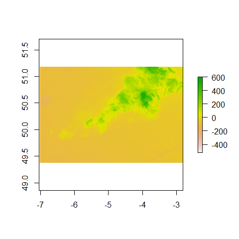
4.4 Raster operations
The raster package provides a variety of functions to perform common GIS operations
on your raster data:
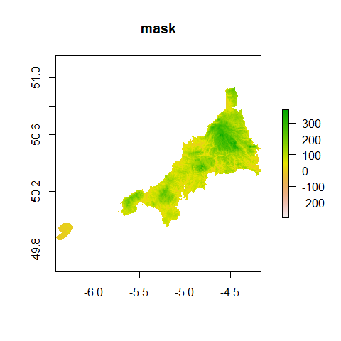
Firstly, there is mask:
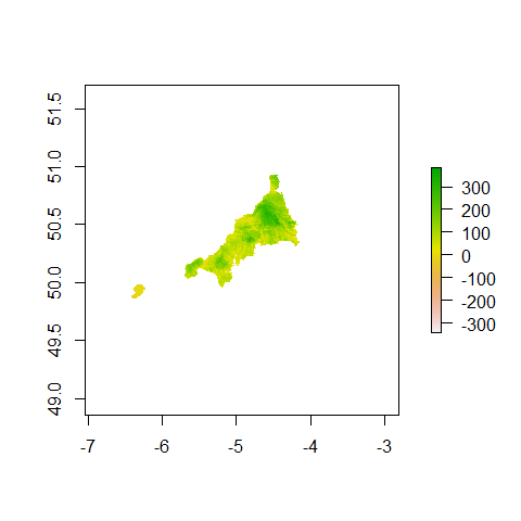
And then there is crop:
This can be reprojected:
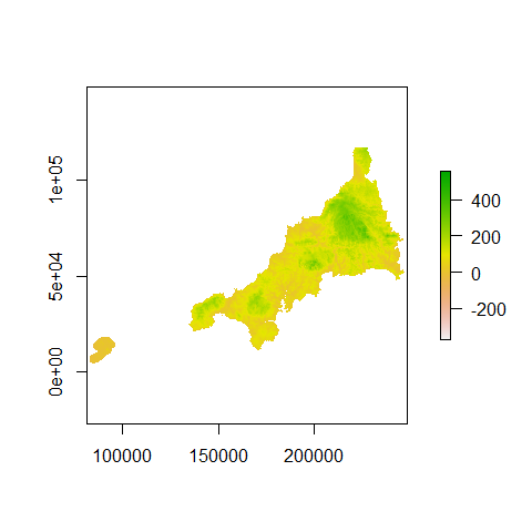
This current elev_cwl_BNG file is an odd spatial resolution so we want to make
give it regular 100 m square cells. This can be done with resample:
## class : RasterLayer
## dimensions : 1303, 1714, 2233342 (nrow, ncol, ncell)
## resolution : 97.3, 97.5 (x, y)
## extent : 81662.17, 248434.4, -2593.72, 124448.8 (xmin, xmax, ymin, ymax)
## crs : +proj=tmerc +lat_0=49 +lon_0=-2 +k=0.9996012717 +x_0=400000 +y_0=-100000 +datum=OSGB36 +units=m +no_defs +ellps=airy +towgs84=446.448,-125.157,542.060,0.1502,0.2470,0.8421,-20.4894
## source : memory
## names : layer
## values : -371.462, 819.7913 (min, max)tmpR <- raster(nrow=1271,ncol=1669)
crs(tmpR) <- crs(cwl)
extent(tmpR) <- c(81600,248500,-2600,124500)
elev_100m <- resample(elev_cwl_BNG, tmpR)
plot(elev_100m,main="100 m")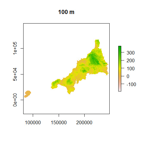
Let’s remove the Isles of Scilly with the extract function.
Firstly, we need to find some coordinates that fall between the Isles of Scilly
(westernmost data) and the mainland AND south of Lizard Point (southernmost mainland).
Use the locator function to interact with the plot window. Click ``Finished’’
in the top right corner when you are done to view the coordinates in console:
Now we can take those coordinates and round them to the nearest 100 m:
# For example you could try this... but give the locator() tool a go
e_crop <- c(129000, 248500, 1600, 124500) # xmin, xmax, ymin, ymax
# Now crop
crop_elev_100m <- crop(elev_100m, e_crop)
plot(crop_elev_100m, main="crop")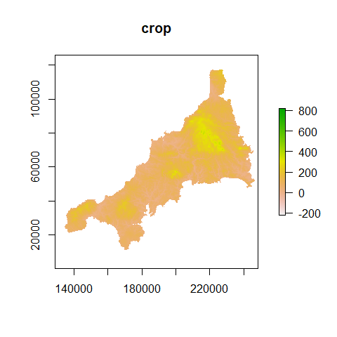
# Let's convert this back to WGS84
elev_100m_WGS84 <- projectRaster(crop_elev_100m, crs = crs(wgs84))
plot(elev_100m_WGS84, main="100 m WGS84")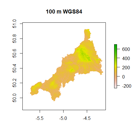
Another operation called aggregate allows us to reduce the spatial resolution:
elev_1000m <- aggregate(crop_elev_100m,10,fun=mean,expand=TRUE, na.rm=TRUE)
plot(elev_1000m, main = "1000 m")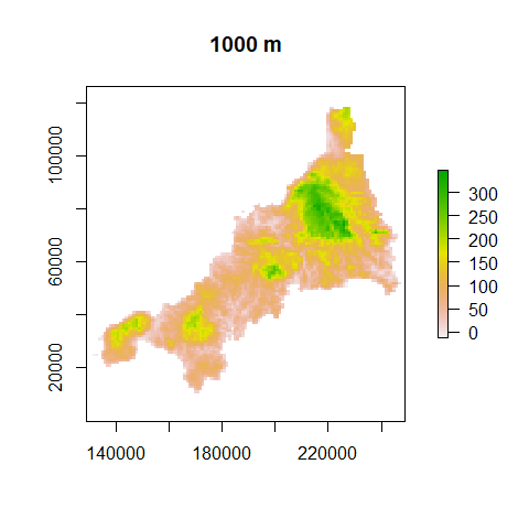
4.5 Raster Manipulation
4.5.1 Raster maths
Simple raster maths or ‘map algebra’ can be done as per the example below but it can get much more complicated. When using another raster to perform an operation in your raster math, both rasters must have the same extent and resolution:
The cellStats function is useful for finding broad statistics about a layer
e.g. sum, mean, min, max, sd, ‘skew’ and ‘rms’ of which the latter two must be
supplied as a character value (with quotes):
## [1] 108.59684.5.2 Terrain models
Quite often, much more information can be obtained from raster data, by looking at the relationship between a cell and it’s neighbours. Topographical indices such as slope and aspect can be obtained by using a single function with our elevation data:
models <- terrain(elev_100m_WGS84, opt=c("slope", "aspect", "TPI", "TRI",
"roughness", "flowdir"), unit='degrees')
class(models)## [1] "RasterBrick"
## attr(,"package")
## [1] "raster"## class : RasterBrick
## dimensions : 1293, 1251, 1617543, 6 (nrow, ncol, ncell, nlayers)
## resolution : 0.00141, 0.000898 (x, y)
## extent : -5.867338, -4.103428, 49.84596, 51.00708 (xmin, xmax, ymin, ymax)
## crs : +proj=longlat +datum=WGS84 +ellps=WGS84 +towgs84=0,0,0
## source : memory
## names : tri, tpi, roughness, slope, aspect, flowdir
## min values : 2.289150e-02, -1.178207e+02, 0.000000e+00, 4.132828e-03, 6.612837e-04, 1.000000e+00
## max values : 244.5606, 122.4477, 705.7529, 67.0107, 359.9989, 128.0000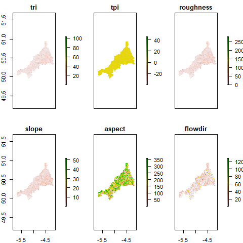
4.5.3 Hillshade
We can also make a hillshade raster and overlay the elevation data. We introduce
a way of subsetting the raster stack/brick here using subset but you could
also use slope <- models$slope or other means we introduced at the beginning
of this section:
slope <- subset(models, "slope") # select slope
aspect <- subset(models, "aspect") # select slope
hill <- hillShade(slope, aspect, 45, 270)
plot(hill, col = grey(0:100/100), legend = FALSE)
plot(elev_100m_WGS84, col = rainbow(25, alpha=0.35), add=TRUE)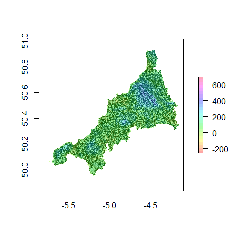
4.6 Visualisation
4.6.1 Create a map
Maps can be quickly created using leaflet and basemaps from OpenStreetMap
or tiles from MapBox imagery can be imported to enhance the map:
pal <- colorNumeric(c("#FFFFCC", "#41B6C4", "#0C2C84"), domain=c(0,500, na.rm=T),
na.color = "transparent", reverse = T)
leaflet() %>%
addTiles() %>% # OpenStreetMap base map
addRasterImage(elev_100m_WGS84, colors = pal, opacity = 0.8) %>%
addLegend(pal = pal, values = c(0, 500),
title = "Cornwall Elevation")## Warning in colors(.): Some values were outside the color scale and will be
## treated as NAleaflet package is highly versatile and can do a lot more.
You can explore more here.
4.6.2 Visualize in 3D
We can also make an interative 3D plot of a RasterLayer. You can modifiy several parameters like the color palette or the elevation scale relative to x and y.