2 Linear models

Slides can be downloaded from:

• LMs in R

2.1 Simple linear regression

In many scientific applications we are interested in exploring the relationship between a single response variable and multiple explanatory variables (predictors). We can do this by fitting a linear model. Linear models per se do not infer causality, i.e defining a variable as response or explanatory is somewhat arbitrary and depends on what the researcher is interested in. Causality can however be inferred through careful experimental design in a well-controlled setting.

Consider again the case of one response and one explanatory variable. From the previous chapter we know that this boils down to the equation of a line (\(y = mx +c\)). Let’s rename the parameters \(c\) and \(m\) to \(\beta_0\) and \(\beta_1\), in line with statistical naming convention¹. It is just a change in name:

\[ \begin{aligned} y = c + mx\\ y = \beta_0 + \beta_1x \end{aligned} \]

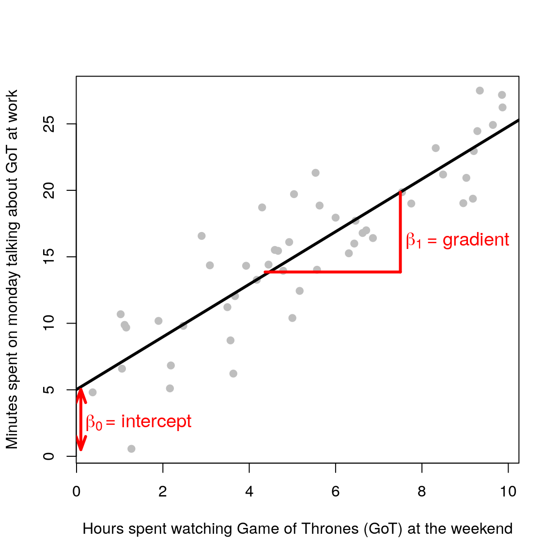
Now suppose we measure \(n\) independent and identically distributed (i.i.d) normally distributed outcomes \(y_1,\ldots,y_n\) (e.g height of people) and we want to model their relationship with some explanatory variable \(x\) (e.g weight of people). The linear regression model is defined as follows:

\[ \begin{aligned} y_i & = \beta_0 + \beta_1x_i + \epsilon_i \\ \epsilon_i & \sim \mathcal{N}(0, \sigma^2) \end{aligned} \] \(i\) is an index that goes from 1 to \(n\) (the total number of observations). The equation is the same as before (\(y = \beta_0 + \beta_1x\)), but now we have added an error term \(\epsilon\). This term is needed because the straight line cannot go through all the data points (unless you have a very questionable dataset)! It represents the discrepancy between the model (the fitted straight line) and the observed data (grey points).

\(\epsilon\) is also known as the noise term. The reason is that in general our response variable has some uncertainty associated with it (e.g counting the number of birds in an area, quantifying gene expression using microarrays or RNA-seq, etc.). The statistical assumption in linear modelling is that these errors are normally distributed with mean zero and some standard deviation \(\sigma\) (mathematically this is written as \(\epsilon_i \sim \mathcal{N}(0, \sigma^2)\)). This means that the response variable is also assumed to be normally distributed. For the maths aficionados amongst you:

\[ y_i \sim \mathcal{N}(\beta_0 + \beta_1x_i, \sigma^2) \] Note that we do not make explicit assumptions about the explanatory variables (the \(x\)’s) i.e they don’t need to be normal.

The workflow in linear regression is as follows:

1. Infer the model’s parameters \(\beta_0\) and \(\beta_1\).
2. Check the model fit.
3. Interpret the practical significance of the estimated parameters.

2.2 Doing it in R

Luckily for us, we do not need to worry about the mathematical intricacies of estimating the model’s parameters, R will do it for us. Let’s generate some fake data just to get things started.

set.seed(1453)
N <- 100 ## no. of observations
weight <- runif(n=N, min=60, max=100) ## hypothetical weights in kg
height <- 2.2*weight + rnorm(n=N, mean=0, sd=10) ## hypothetical heights in cm
plot(weight, height, pch=19, xlab='Weight (kg)', ylab='Height (cm)', col='grey')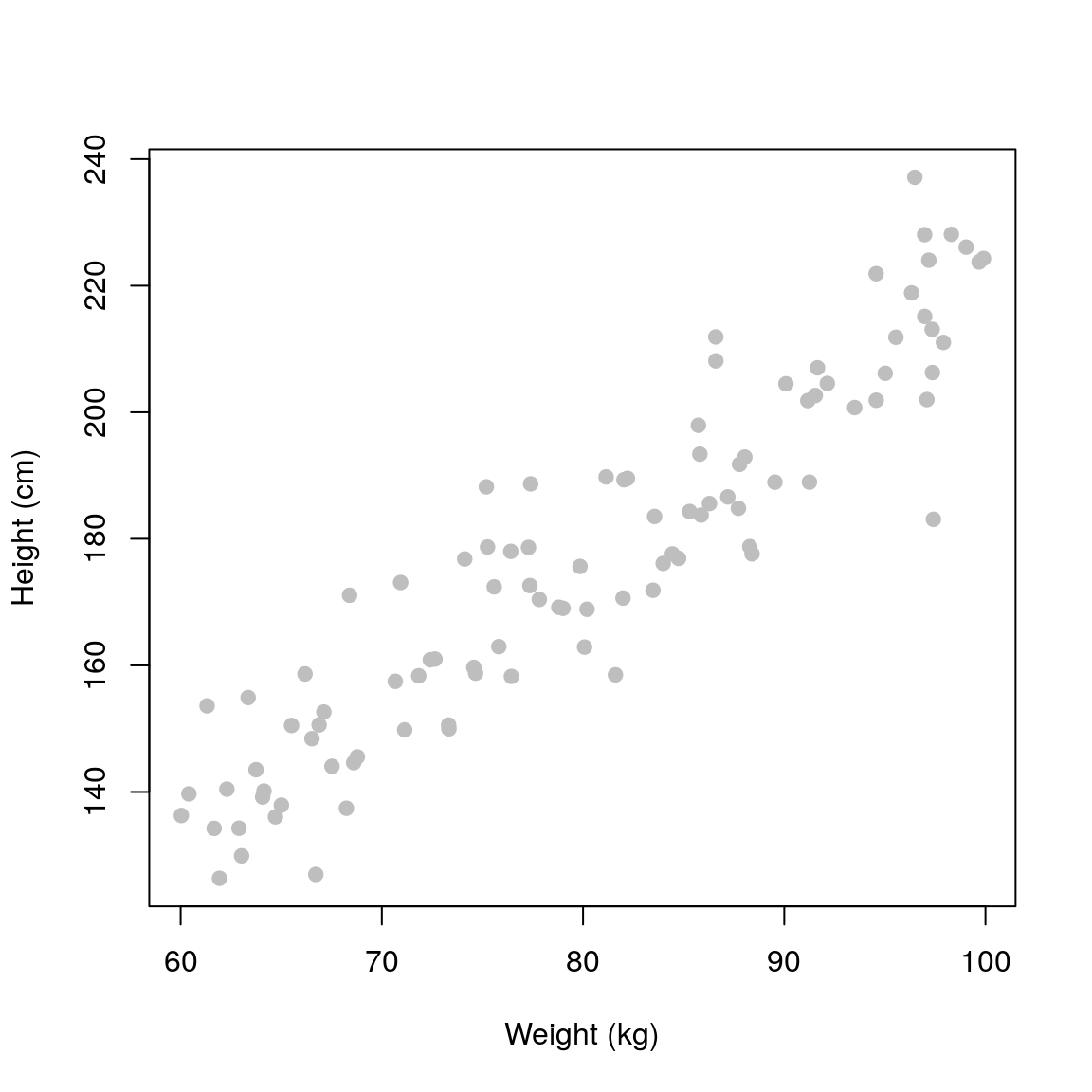

To fit a linear model we use the lm() function (always read the documentation of a function before using it!). This function requires a formula object which has the form of response ~ explanatory. So in our case this will be height ~ weight. R will then fit the following model ²:

\[ \mathrm{height}_i = \beta_0 + \beta_1\mathrm{weight}_i + \epsilon_i \] Let’s call the R function, plot the model fit and print the output.

## Linear model fit
fit <- lm(height ~ weight)

## Plot model fit
plot(weight, height, pch=19, xlab='Weight (kg)', ylab='Height (cm)', col='grey')
lines(weight, predict(fit), col='black', lwd=3)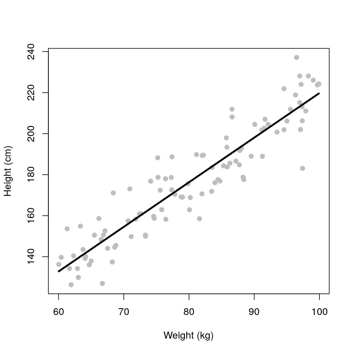

## Print result
print(fit)

## 
## Call:
## lm(formula = height ~ weight)
## 
## Coefficients:
## (Intercept)       weight  
##       2.352        2.174

This outputs two numbers, the (Intercept)= 2.352 cm and weight= 2.174 cm/kg. These are the \(\beta_0\) and \(\beta_1\) parameters.

The \(\beta_0\) parameter (intercept) is not very useful in this case, it basically tells us what’s the expected height of someone that weighs 0 kg (2.352 cm here). This is of course nonsense, but I’m highlighting it as a reminder that the assumptions that underlie these models can only be tested within the range of the observed data.

Aside: using the model to predict outside of the range of the observed data is called extrapolating. Oftentimes, statistical models are developed in order to be used to extrapolate (e.g. climate modelling). This is however, dangerous, as we can only assess the assumptions of the model over the range of the observed data. When extrapolating we have to assume that these relationships hold beyond the range of the data, which may or may not be reasonable (hence why weather forecast over short-time periods are OK, but climate forecasts are much more uncertain). Hence, we should always view the model as an approximation of the data generating process. In this particualr case, the interpretation of the parameters is not sensible when \(x = 0\) (weight = 0 kg), but makes sense in the range that we are interested in exploring. If the case where \(x = 0\) is important, then we would have to change the model to ensure that the predictions made sense at those values of \(x\).

The \(\beta_1\) parameter (gradient) tells us about the relationship between the outcome and explanatory variable. In this case, for every 1 kg increase in weight on average the height increases by 2.174 cm.

Warning: the notation used by R can come across as confusing. Although the returned value is labelled as weight, in fact it corresponds to the \(\beta_1\) parameter that relates to the strength of linear relationship between weight and height (i.e it is a gradient).

2.2.1 Using data frames

The lm() function also accepts data frames as input arguments.

## Create data frame
df <- data.frame(height=height, weight=weight)
head(df)

##     height   weight
## 1 211.9054 86.59694
## 2 178.6420 77.28891
## 3 206.1585 95.01870
## 4 157.4803 70.66759
## 5 175.6296 79.84837
## 6 176.1113 83.98290

## Fit linear model
fit <- lm(height ~ weight, data=df)

2.2.2 Extended summary

The object returned by lm() contains further information that we can display using the summary() function.

summary(fit)

## 
## Call:
## lm(formula = height ~ weight, data = df)
## 
## Residuals:
##     Min      1Q  Median      3Q     Max 
## -31.089  -6.926  -0.689   6.057  24.967 
## 
## Coefficients:
##             Estimate Std. Error t value Pr(>|t|)    
## (Intercept)  2.35229    7.11668   0.331    0.742    
## weight       2.17446    0.08782  24.762   <2e-16 ***
## ---
## Signif. codes:  0 '***' 0.001 '**' 0.01 '*' 0.05 '.' 0.1 ' ' 1
## 
## Residual standard error: 10.31 on 98 degrees of freedom
## Multiple R-squared:  0.8622, Adjusted R-squared:  0.8608 
## F-statistic: 613.1 on 1 and 98 DF,  p-value: < 2.2e-16

That’s a lot of information, let’s unpick it line by line:

• Call

  This just states the arguments that were passed to the lm() function. Remember it’s response ~ explanatory.

• Residuals

  Some basic stats about the residuals (i.e the differences between the model fit and the observed data points). It is easier to plot a histogram of the residuals (shown in the next section), but these basic stats can already give us an indication of whether we have a symmetric distribution with zero mean (i.e we want the median to be close to zero, the third quartile (3Q) to be roughly equal to -1Q (first quartile) and the max to be approximately -min).

• Coefficients
  • Estimate

  The (Intercept)= 2.352 cm and weight= 2.174 cm/kg are the \(\beta_0\) and \(\beta_1\) parameters as discussed earlier.

  • Std. Error

  The standard error for that parameter. It tells us how confident we are in estimating that particular parameter. If the standard error is comparable or greater than the actual parameter estimate itself then that point estimate should not be trusted. We can also show the confidence intervals for the model parameters to highlight their uncertainty using the confint() function:

  confint(fit, level=0.97) ## pick the 97% confidence intervals

  ##                  1.5 %    98.5 %
  ## (Intercept) -13.319698 18.024268
  ## weight        1.981077  2.367844

  • t value and Pr(>|t|)

  This is the result of a hypothesis testing against the null hypothesis that the coefficient is zero.

• Residual standard error

  The square root of residual sum of squares/degress of freedom

  ## Residual standard error
  sqrt(sum(residuals(fit)^2) / fit$df.residual) 

  ## [1] 10.31254

• Multiple R-squared

  Total variation = Regression (explained) variation + Residual (unexplained) variation

  The \(R^2\) statistic (also known as the coefficient of determination) is the proportion of the total variation that is explained by the regression. In regression with a single explanatory variable, this is the same as the Pearson correlation coefficient squared:

  cor(height, weight)^2

  ## [1] 0.8621921

• F-statistic

  \[ \text{F-statistic} = \frac{\text{Regression (explained) variation}}{\text{Residual (unexplained) variation}} \]

  The F-statistic can be used to assess whether the amount of variation explained by the regression (\(M_1\)) is statistically significantly different compared to the null model (\(M_0\) - in this case the null model is the same as just taking the mean of the data). Large values of the F-statistic correspond to cases where the model fit is better for the more complex model compared to the null model. This test can be used to generate a p-value to assess whether the model fit is statistically significantly better given a pre-defined level of significance.

  \[ \begin{aligned} M_0:~~~~~y_i &= \beta_0 + \epsilon_i\\ M_1:~~~~~y_i &= \beta_0 + \beta_1 W_i + \epsilon_i \end{aligned} \]

2.3 Model checking

The extended summary leads us nicely to the concept of model checking. In theory, we can fit an infinite number of different models to the same data by placing different assumptions/constraints. Recall:

All models are wrong but some are useful - George E.P. Box

In order to make robust inference, we must check the model fit

Model checking boils down to confirming whether or not the assumptions that we have placed on the model are reasonable. Our main assumption is that the residuals are normally distributed centred around zero. Let’s plot this:

hist(fit$residuals)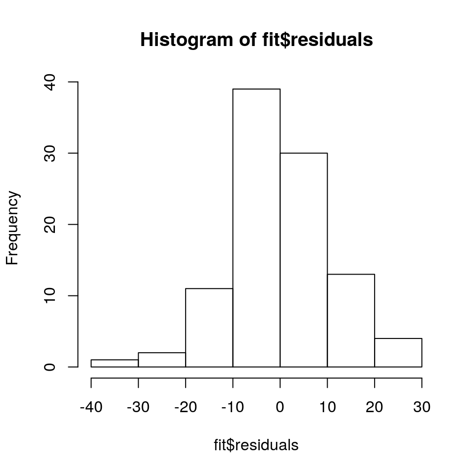

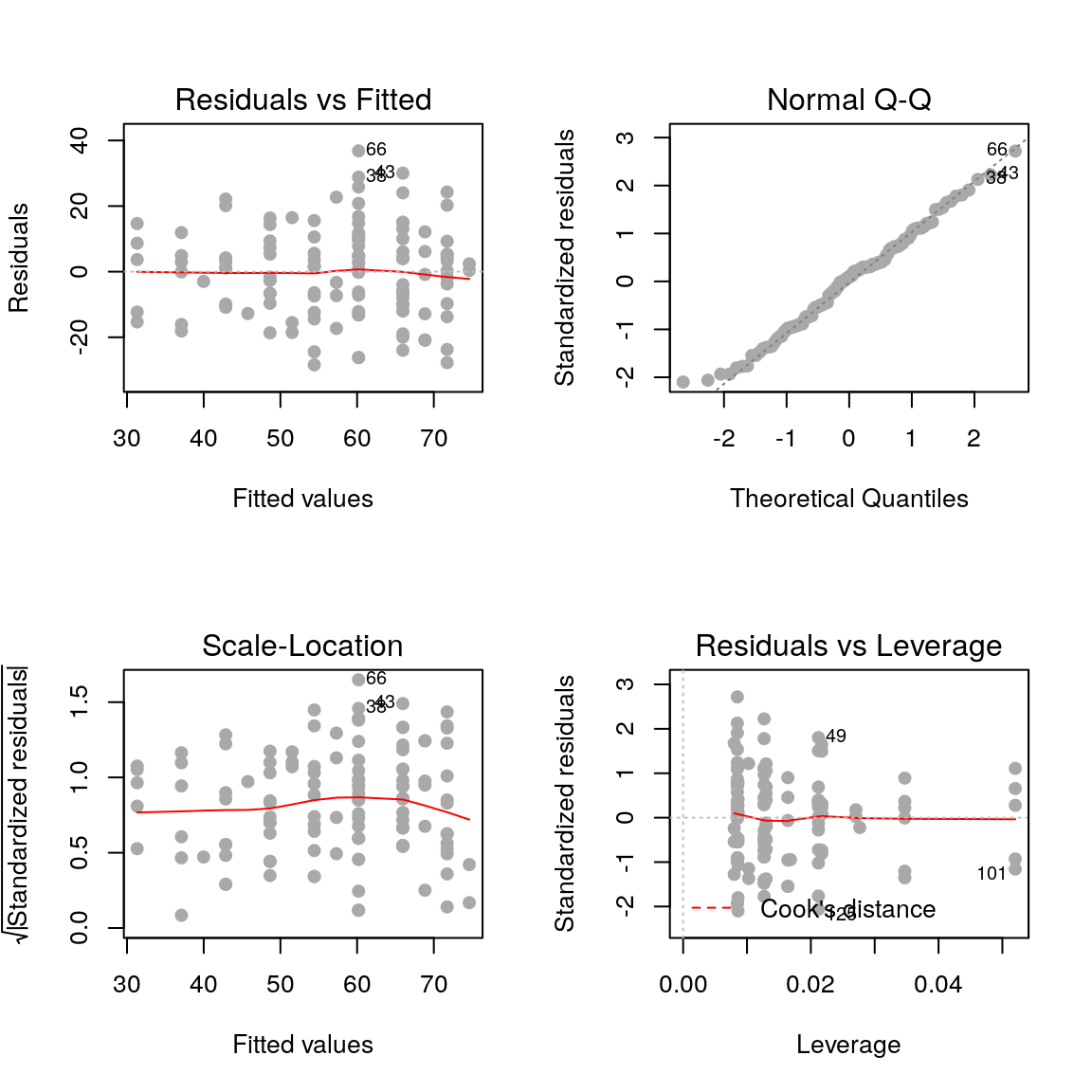
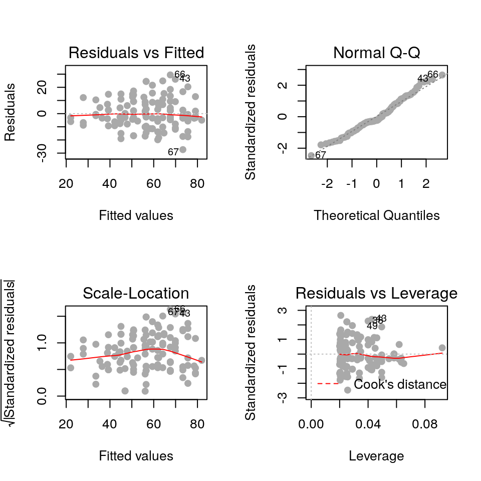
The residuals are fairly normally distributed which is a good sign. R also provides us with the following diagnostic plots:

par(mfrow=c(2, 2))
plot(fit, pch=19, col='darkgrey')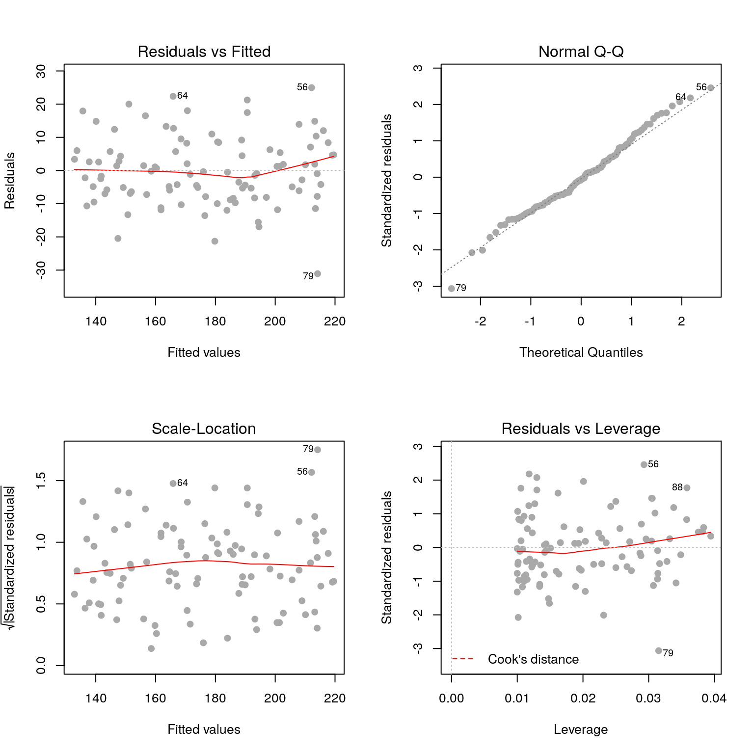

2.3.1 Residuals vs fitted values

plot(fit, pch=19, col='darkgrey', which=1)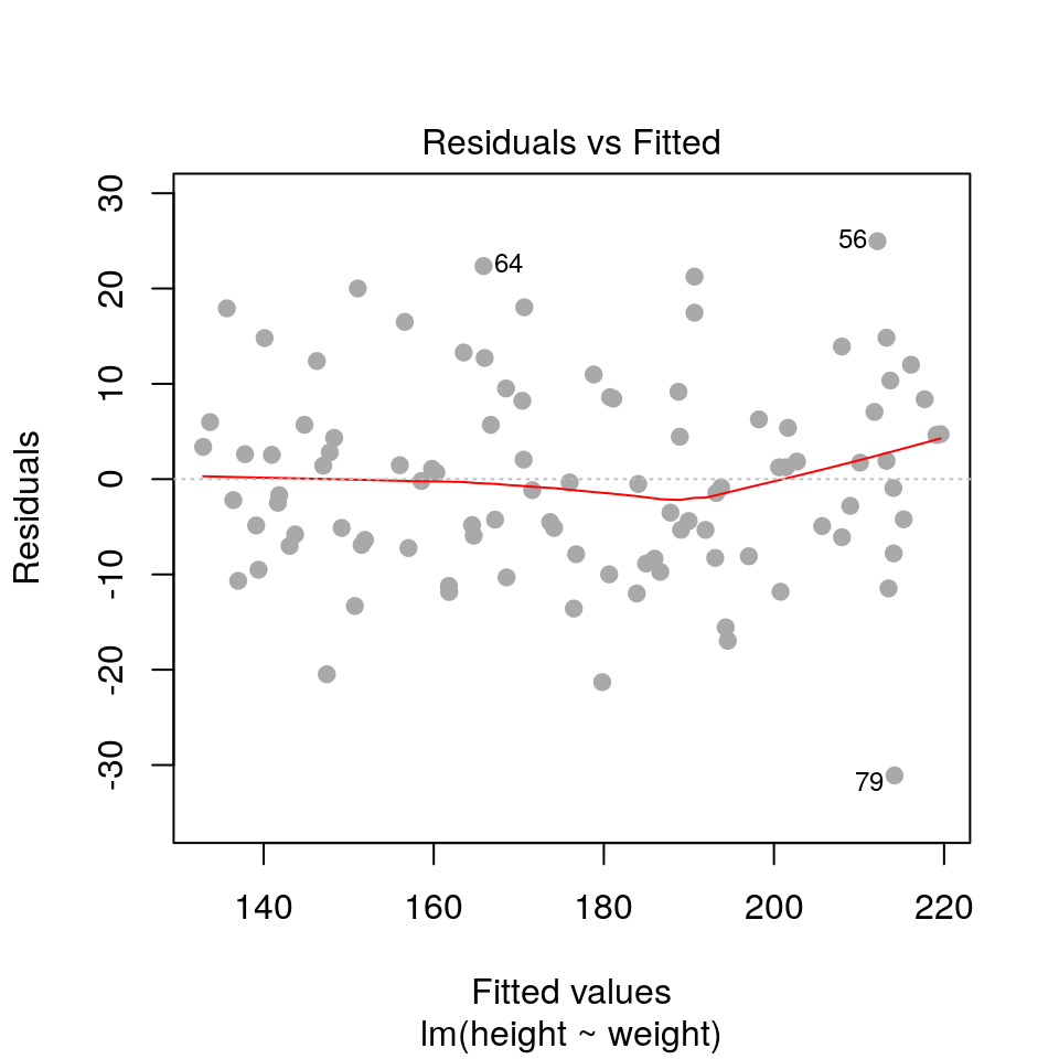

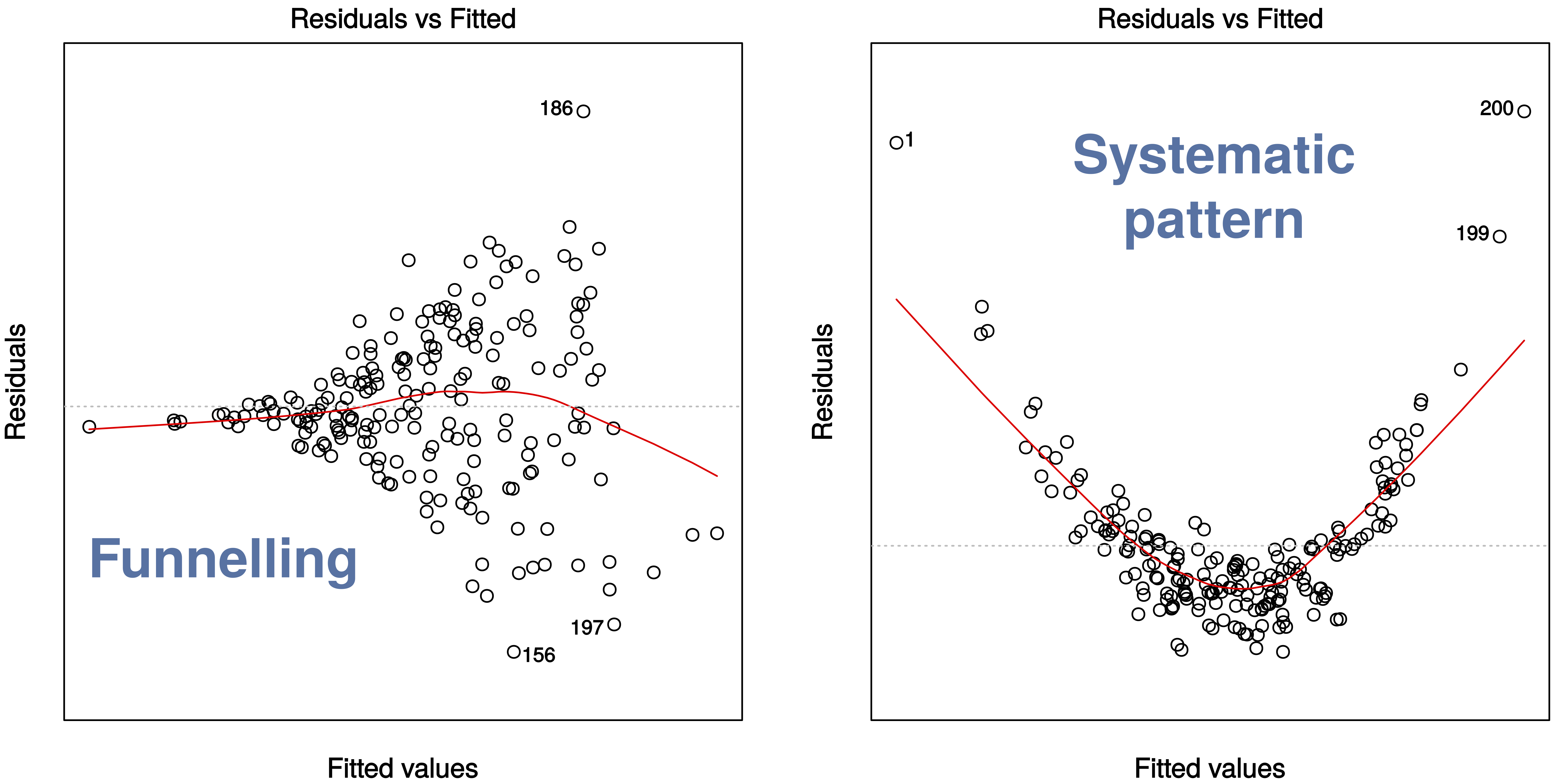
Here we are checking that the variance is constant along the fitted line³, and that there are no systematic patterns in the residuals.

A couple of example where this assumption is violated.

2.3.2 Residuals vs fitted values (scale-location)

plot(fit, pch=19, col='darkgrey', which=3)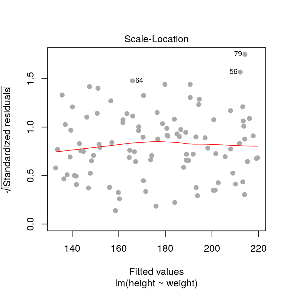

This is similar to the first plot but on a different scale.

2.3.3 Residuals vs. leverage

plot(fit, pch=19, col='darkgrey', which=5)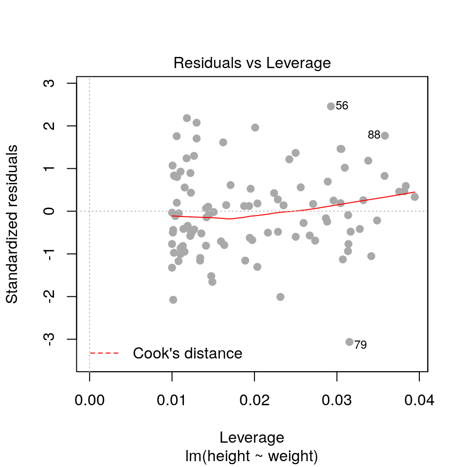

• Leverage: a measure of how isolated individual points are in relation to other points
• Cook’s Distance: a measure of how influential a point is to the regression

These measures help us identify potential outliers.

2.3.4 QQ plots

plot(fit, pch=19, col='darkgrey', which=2)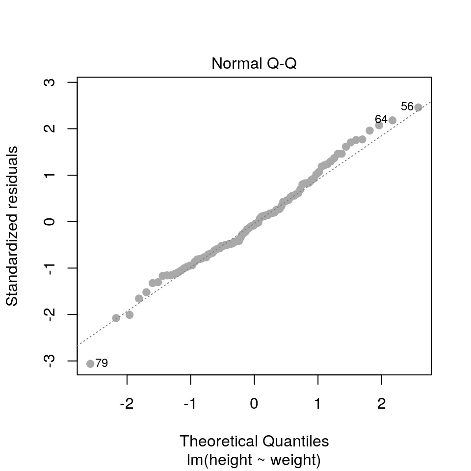

Here we are checking that the assumption of normally distributed errors is reasonable. Points should follow the dashed line.

2.4 Practical 1

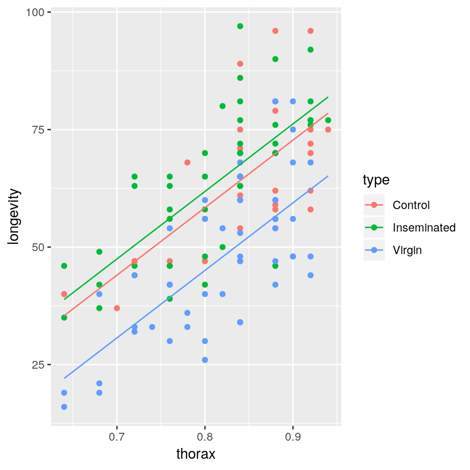
We will use the fruitfly dataset (Partridge and Farquhar (1981)) introduced in the “Advanced Visualisation and Data Wrangling in R”, which is summarised again here (do not worry about the details of the study for now, this is only included for the sake of completeness):

A cost of increased reproduction in terms of reduced longevity has been shown for female fruitflies, but not for males. We have data from an experiment that used a factorial design to assess whether increased sexual activity affected the lifespan of male fruitflies.

The flies used were an outbred stock. Sexual activity was manipulated by supplying individual males with one or eight receptive virgin females per day. The longevity of these males was compared with that of two control types. The first control consisted of two sets of individual males kept with one or eight newly inseminated females. Newly inseminated females will not usually remate for at least two days, and thus served as a control for any effect of competition with the male for food or space. The second control was a set of individual males kept with no females. There were 25 males in each of the five groups, which were treated identically in number of anaesthetisations (using \(\mathrm{CO}_2\)) and provision of fresh food medium.

Download the data file from here and save it to your working directory.

Since we are working with data.frame() objects, where appropriate, we have provided examples using both base R or tidyverse (for those of you who attended the Advanced Visualisation and Data Wrangling workshop).

ff <- readRDS("fruitfly.rds")

head(ff)

##   partners        type longevity thorax sleep
## 1        8 Inseminated        35   0.64    22
## 2        8 Inseminated        37   0.68     9
## 3        8 Inseminated        49   0.68    49
## 4        8 Inseminated        46   0.72     1
## 5        8 Inseminated        63   0.72    23
## 6        8 Inseminated        39   0.76    83

For the purpose of this practical we will assume that the no female case is the control case, whilst the inseminated and virgin female cases are the treatment cases.

• partners: number of companions (0, 1 or 8)
• type: type of companion (inseminated female; virgin female; control (when partners = 0))
• longevity: lifespan, in days
• thorax: length of thorax, in mm
• sleep: percentage of each day spent sleeping

Task

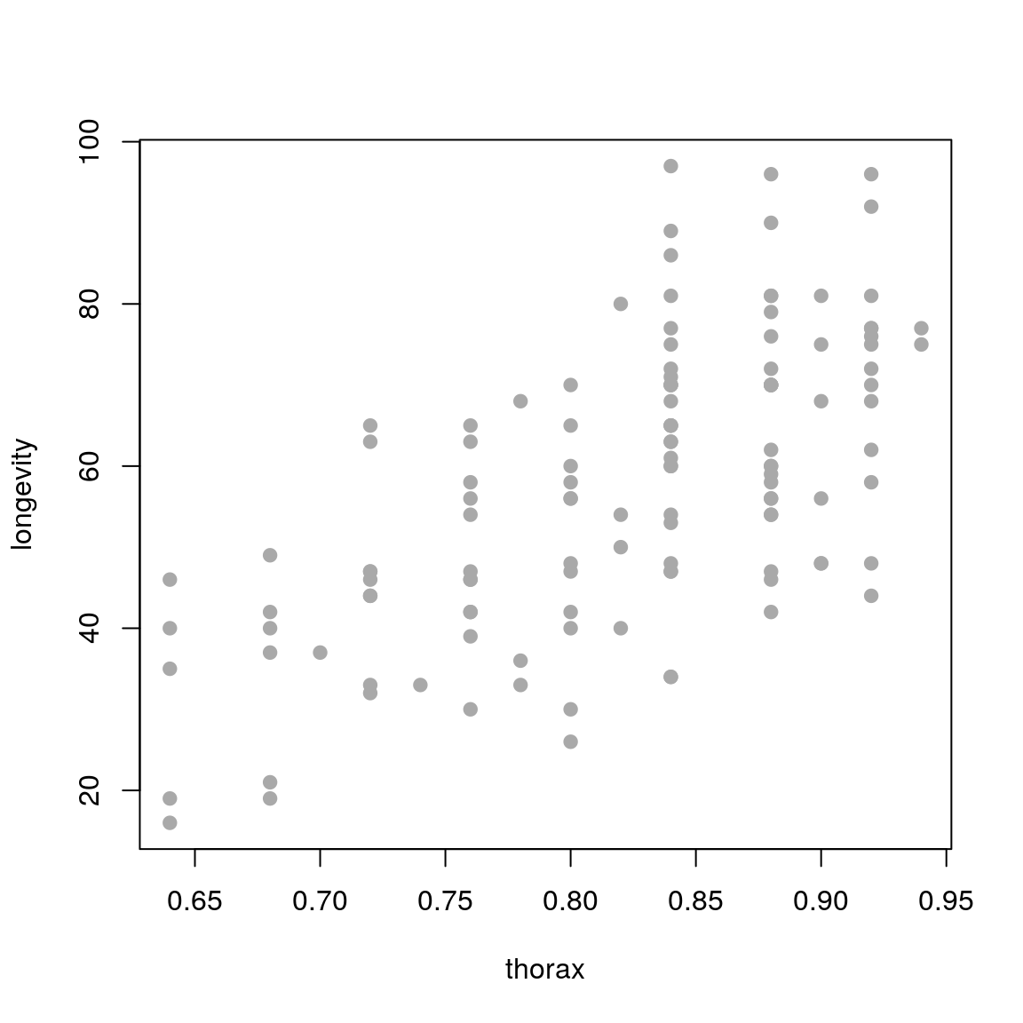
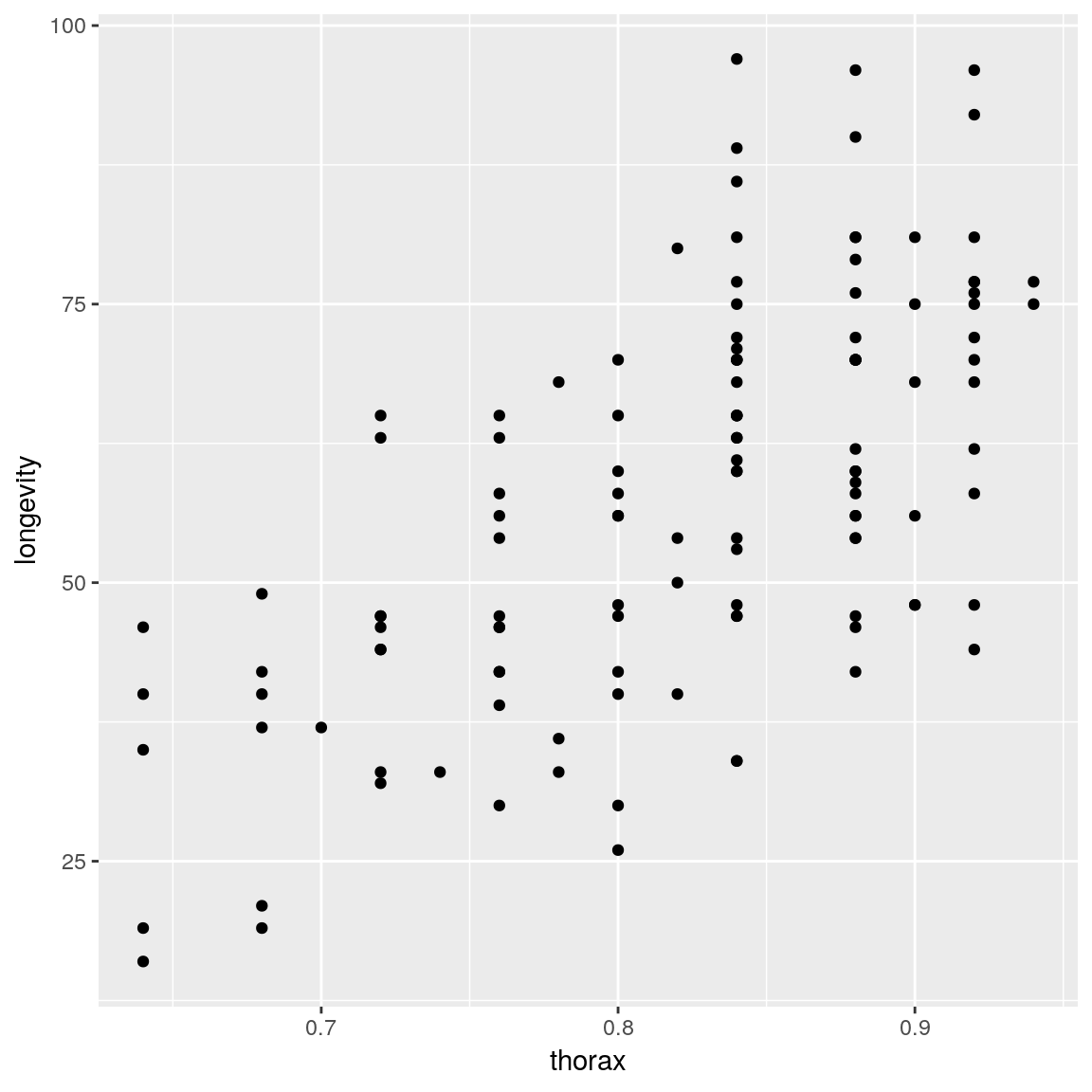
Produce a scatterplot of longevity against thorax. What does the relationship look like?

Solution

plot(longevity ~ thorax, data = ff, 
     pch=19, col='darkgrey')

The plot suggests that a linear relationship might exist between the two variables. So we can proceed by fitting a linear model in R.

ggplot(ff) +
    geom_point(aes(x = thorax, y = longevity))

The plot suggests that a linear relationship might exist between the two variables. So we can proceed by fitting a linear model in R.

Task

1. Fit a linear model with lifespan as response variable and thorax length as explanatory variable.
2. Display a summary of the fit, together with the 97% confidence interval for the estimated parameters.
3. Show the diagnostic plots for the model.

Solution

fit <- lm(longevity ~ thorax, ff)
summary(fit)

## 
## Call:
## lm(formula = longevity ~ thorax, data = ff)
## 
## Residuals:
##     Min      1Q  Median      3Q     Max 
## -28.415  -9.961   1.132   9.265  36.812 
## 
## Coefficients:
##             Estimate Std. Error t value Pr(>|t|)    
## (Intercept)   -61.05      13.00  -4.695  7.0e-06 ***
## thorax        144.33      15.77   9.152  1.5e-15 ***
## ---
## Signif. codes:  0 '***' 0.001 '**' 0.01 '*' 0.05 '.' 0.1 ' ' 1
## 
## Residual standard error: 13.6 on 123 degrees of freedom
## Multiple R-squared:  0.4051, Adjusted R-squared:  0.4003 
## F-statistic: 83.76 on 1 and 123 DF,  p-value: 1.497e-15

confint(fit, level=0.97)

##                 1.5 %   98.5 %
## (Intercept) -89.60261 -32.5008
## thorax      109.70817 178.9580

par(mfrow=c(2, 2))
plot(fit, pch=19, col='darkgrey')

par(mfrow=c(1, 1))

2.5 Prediction

One of the key benefits of fitting a statistical model is that we can use it to produce predictions of the response variable for new values of the explanatory variable(s). We can do this using the predict() function in R. For example, in the fruitflies example above, we may want to produce estimates of average longevity for given values of thorax. To do this we must create a new data.frame object containing all the values of explanatory variables that we want to use for our prediction.

Note: we only require the explanatory variables in this new data frame, the response variable will be generated from the model.

For example, if we wanted to produce an estimate of longevity for an average individual with a thorax length of 0.8mm, we can run:

## produce predicted longevity for thorax = 0.8mm
newdata <- data.frame(thorax = 0.8)
predict(fit, newdata)

##        1 
## 54.41478

We can also use this to produce confidence or prediction intervals as follows:

## produce predicted longevity for thorax = 0.8mm
newdata <- data.frame(thorax = 0.8)
predict(fit, newdata, interval = "confidence", level = 0.97)

##        fit      lwr      upr
## 1 54.41478 51.64686 57.18269

Note: If you predict without an interval argument, the predict() function returns a vector, otherwise it returns a matrix.

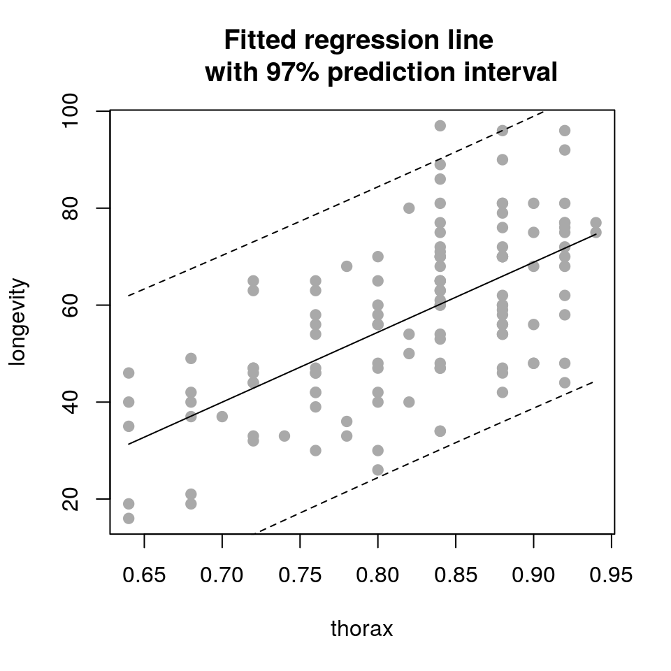
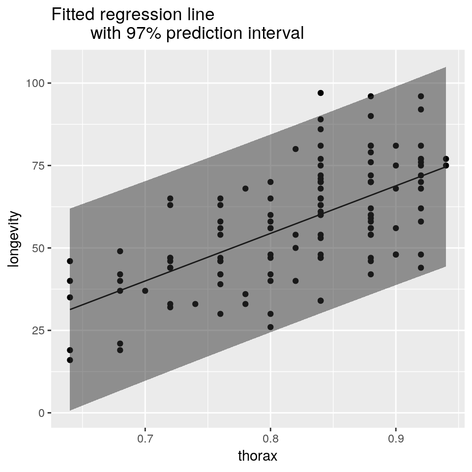
Aside: there are two types of intervals that you might want to produce: confidence or prediction intervals.

• Confidence intervals: these correspond to the uncertainty surrounding our estimate of an average individual (i.e. it represents the uncertainty in the mean: \(y = \beta_0 + \beta_1 x\)
• Prediction intervals: these correspond to the uncertainty surrounding an individual observation: \(y_i = \beta_0 + \beta_1 x_i + \epsilon_i\).

If the model fits well, then we would expect \(100(1 - \alpha)\)% of the individual measurements to lie within the prediction interval, where \(\alpha\) is the significance level (so \(\alpha = 0.03\) corresponds to a 97% confidence interval).

The predict() function can be used as a very general way to produce plots of the fitted values over the observed data. For example, let’s consider that we wish to add our fitted regression line to our observed data plot.

plot(longevity ~ thorax, data = ff, pch = 19, col='darkgrey')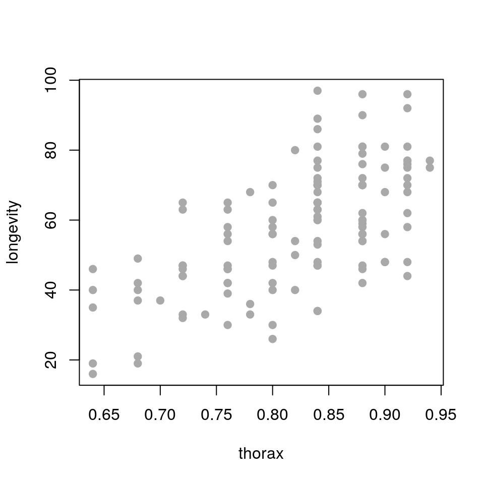

There are various ways to add the correct regression line to this plot, but we will show you a general way that can be used for lots of different types of models. Firstly, we generate a range of \(x\)-coordinates that we wish to predict to e.g.

## create new data frame to predict to
newdata <- data.frame(thorax=seq(min(ff$thorax), max(ff$thorax), length.out=50))

We then have to use the model to predict the mean longevity at each of these thorax values:

## predict longevity form the model
newdata <- cbind(newdata, longevity=predict(fit, newdata))

Just as an illustration we will overlay these predictions onto the original scatterplot as points:

## add predicted points to original plot
plot(longevity ~ thorax, data = ff, pch = 19, col='darkgrey')
points(longevity ~ thorax, data = newdata, pch = 19, col = "red")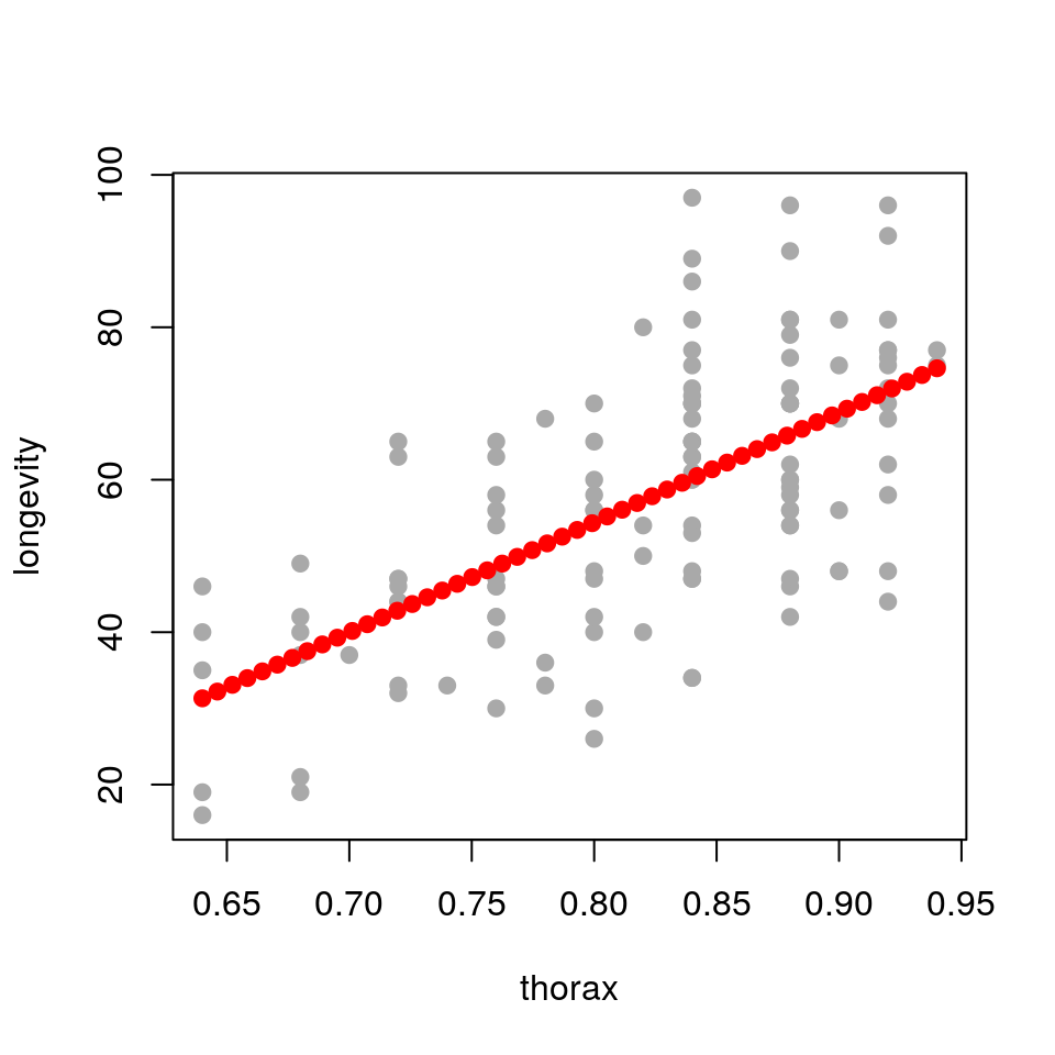

So we have used the predict() function to produce predicted coordinates that we can overlay on the original scatterplot. In practice we would usually plot these predictions as a line rather than points. This approach is particularly useful if the predictions that we wish to plot are not straight lines (such as when we generate confidence or prediction intervals). To complete this example we will now plot the fitted line and associated confidence interval as follows:

## create new data frame to predict to
newdata <- data.frame(thorax=seq(min(ff$thorax), max(ff$thorax), length.out=50))

## produce predictions and intervals
newdata <- cbind(newdata, predict(fit, newdata, interval="confidence", level=0.97))
newdata$longevity <- newdata$fit
newdata$fit <- NULL

## plot fitted line against the raw data
plot(longevity ~ thorax, data = ff, 
     pch = 19, col='darkgrey',
     main = "Fitted regression line
     with 97% confidence interval")
lines(longevity ~ thorax, data = newdata)
lines(lwr ~ thorax, data = newdata, lty = 2)
lines(upr ~ thorax, data = newdata, lty = 2)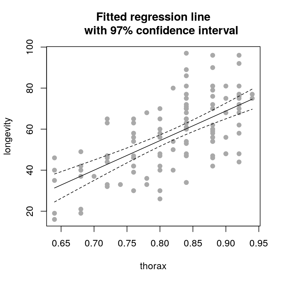

## plot fitted line against the raw data
ggplot(mapping = 
        aes(x = thorax, y = longevity)) +
    geom_point(data = ff) +
    geom_line(data = newdata) +
    geom_ribbon(
        aes(ymin = lwr, ymax = upr), 
        data = newdata, alpha = 0.5)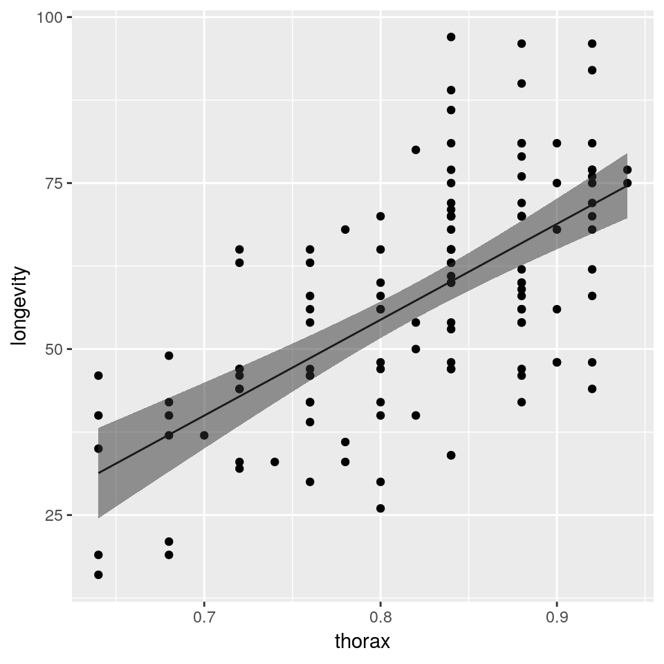

Task

Produce the same plot but with a 97% prediction interval

Solution

## create new data frame to predict to
newdata <- data.frame(
    thorax = seq(min(ff$thorax), 
        max(ff$thorax), length.out = 50)
)

## produce predictions and intervals
newdata <- cbind(newdata, 
    predict(fit, newdata, 
        interval = "prediction", 
        level = 0.97))
newdata$longevity <- newdata$fit
newdata$fit <- NULL

## plot fitted line against the raw data
plot(longevity ~ thorax, data = ff, 
     pch = 19, col='darkgrey',
     main = "Fitted regression line 
     with 97% prediction interval")
lines(longevity ~ thorax, data = newdata)
lines(lwr ~ thorax, data = newdata, 
      lty = 2)
lines(upr ~ thorax, data = newdata, 
      lty = 2)

## create new data frame to predict to
newdata <- data.frame(
    thorax = seq(min(ff$thorax), 
        max(ff$thorax), length.out = 50)
)

## produce predictions and intervals
newdata <- cbind(newdata, 
    predict(fit, newdata, 
        interval = "prediction", 
        level = 0.97)) %>%
    rename(longevity = fit)

## plot fitted line against the raw data
ggplot(mapping = 
        aes(x = thorax, y = longevity)) +
    geom_point(data = ff) +
    geom_line(data = newdata) + 
    geom_ribbon(aes(ymin = lwr, ymax = upr), 
        data = newdata, alpha = 0.5) +
    ggtitle("Fitted regression line
        with 97% prediction interval")

2.6 Multiple linear regression

So far we have looked at examples with one response and one explanatory variable. In most applications we will have several variables that affect our outcome. Extending our simple linear regression model to accommodate multiple explanatory variables is straightforward, we just add them to the model.

Using our illustrative example of height vs weight, let’s add another explanatory variable, for example, the mean height of the individual’s parents (heightParents). Our linear model is defined as follows:

\[ \begin{aligned} y_i & = \beta_0 + \beta_1x_{1i} + \beta_2x_{2i} + \epsilon_i \\ \epsilon_i & \sim \mathcal{N}(0, \sigma^2) \end{aligned} \] Or in English:

\[ \begin{aligned} \mathrm{height}_i & = \beta_0 + \beta_1\mathrm{weight}_i + + \beta_2\mathrm{heightParents}_i+ \epsilon_i \\ \epsilon_i & \sim \mathcal{N}(0, \sigma^2) \end{aligned} \]

Let us make up some data again and plot it.

set.seed(451)

## no. of observations
N <- 100 

## hypothetical weights in kg
weight <- runif(n=N, min=60, max=100) 

## hypothetical mean heights of parents in cm
heightParents <- runif(n=N, min=130, max=210) 

## hypothetical heights in cm
height <- 0.1*weight + 1.05*heightParents + rnorm(n=N, mean=0, sd=10) 

## store as df
df <- data.frame(weight=weight, heightParents=heightParents, height=height) 

## Plot
library(scatterplot3d) ## library needed for 3D plotting
scatterplot3d(weight, heightParents, height, pch=19, xlab='Weight (kg)', 
              ylab='Height of Parents (cm)', zlab='Height (cm)', color='grey')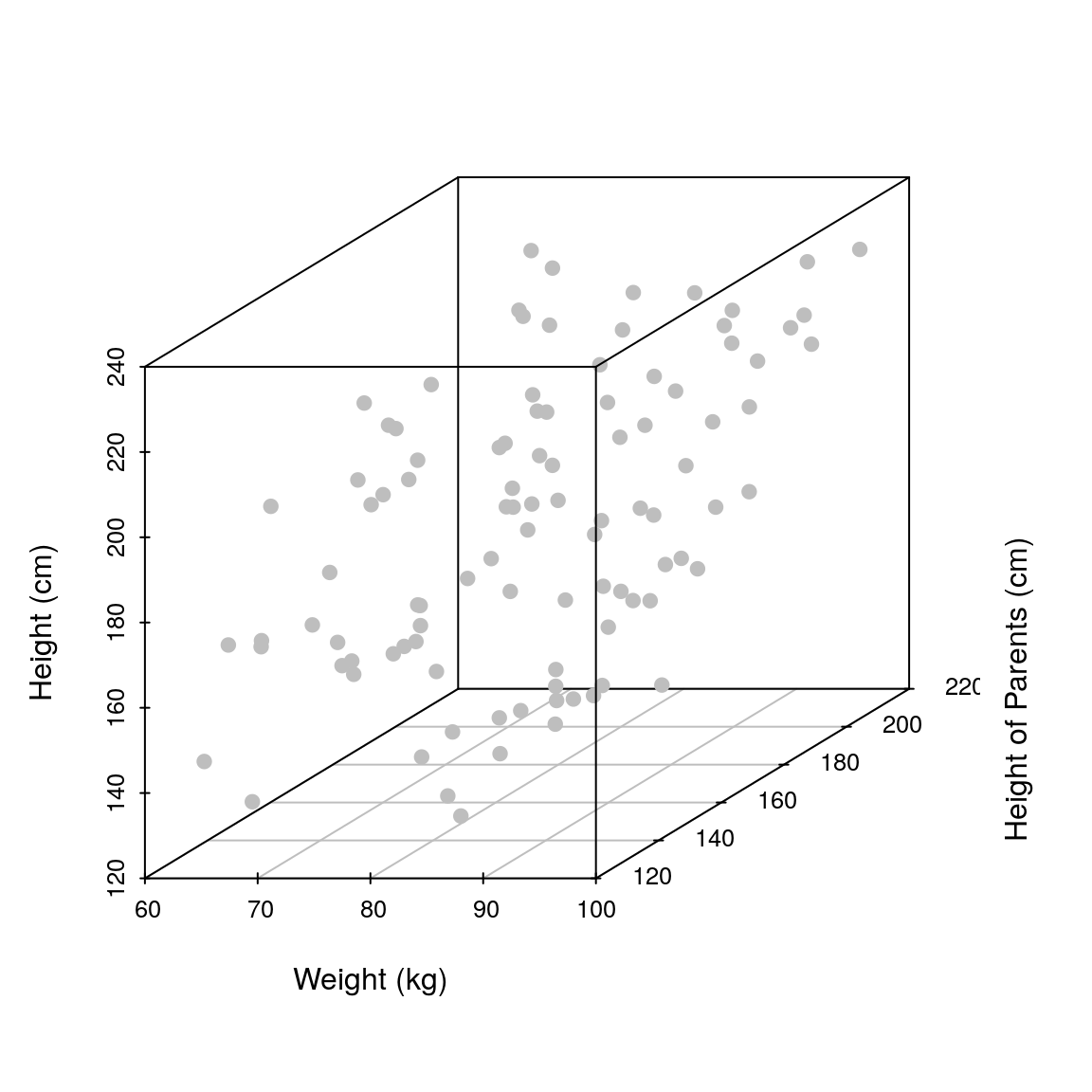

Note how by adding another explanatory variable we are spreading the observations across an additional dimension. That is, we go from a 2D plot to a 3D plot (if we add a third explanatory variable we would need a 4D plot). It is important to keep this in mind; the more explanatory variables we add the more we spread our data thinly across multiple dimensions. In practice, this means that our observations will be sparsely scattered across a high dimensional space, making it hard to fit a robust linear model. In the limit, when we have more explanatory variables than observations, we would not be able to fit a linear model at all (unless we employ a different statistical framework and impose further assumptions/constraints).

The objective of linear modelling is still the same, finding the “best” straight line, or in this case a hyperplane (a line in higher dimensions). You can think of a hyperplane as a (rigid) sheet of paper, where the objective is to place it such that it passes as close as possible to the observed data.

To fit a multiple linear regression model we use the lm() function again and pass the appropriate formula object which has the form of response ~ explanatory_1 + explanatory_2. In in our case this will be height ~ weight + heightParents.

fit <- lm(height ~ weight + heightParents, df)

Let us plot the resultant model first (i.e the hyperplane).

hFig <- scatterplot3d(weight, heightParents, height, pch=19, xlab='Weight (kg)', 
                      ylab='Height of Parents (cm)', zlab='Height (cm)', color='grey')
hFig$plane3d(fit, draw_polygon=TRUE)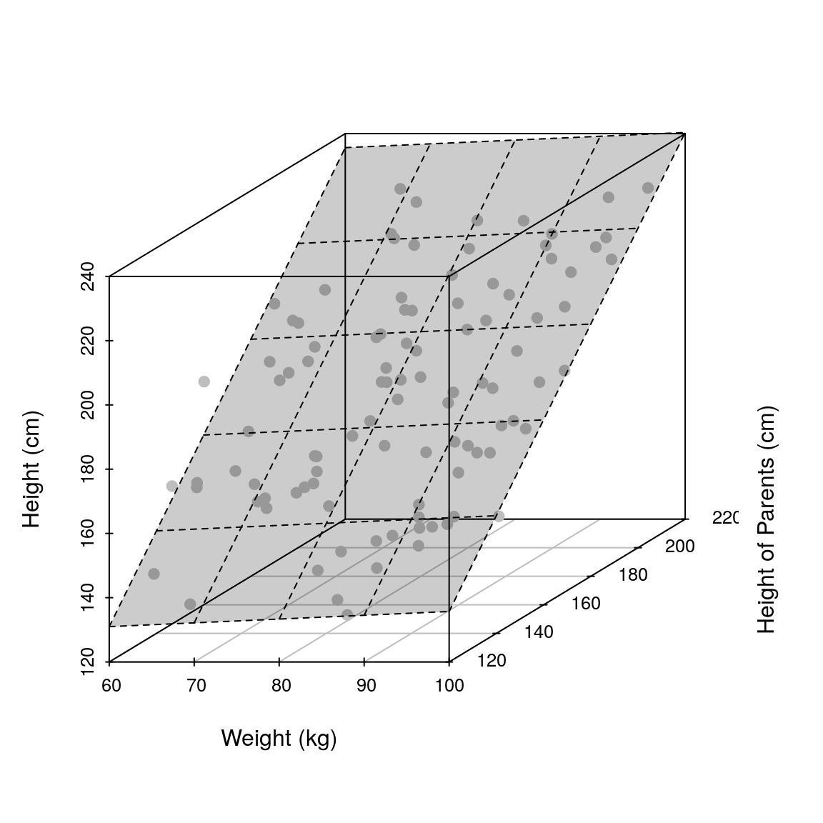

Let us look at the fit’s summary

summary(fit)

## 
## Call:
## lm(formula = height ~ weight + heightParents, data = df)
## 
## Residuals:
##     Min      1Q  Median      3Q     Max 
## -28.578  -6.052   0.235   6.027  27.829 
## 
## Coefficients:
##               Estimate Std. Error t value Pr(>|t|)    
## (Intercept)   -1.65589   10.70833  -0.155    0.877    
## weight         0.11790    0.09198   1.282    0.203    
## heightParents  1.04644    0.04707  22.233   <2e-16 ***
## ---
## Signif. codes:  0 '***' 0.001 '**' 0.01 '*' 0.05 '.' 0.1 ' ' 1
## 
## Residual standard error: 10.19 on 97 degrees of freedom
## Multiple R-squared:  0.8372, Adjusted R-squared:  0.8338 
## F-statistic: 249.4 on 2 and 97 DF,  p-value: < 2.2e-16

Same as before, the (Intercept)= -1.656 cm, weight= 0.1179 cm/kg and heightParents= 1.046 cm/cm are the \(\beta_0\), \(\beta_1\) and \(\beta_2\) parameters.

• The \(\beta_0\) parameter (intercept) is the expected height of someone that weighs 0 kg and whose parents have a mean height of 0 cm. Again, this parameter is not useful in this case.
• The \(\beta_1\) parameter tells us about the relationship between height and weight. For every 1 kg increase in weight on average the height increases by 0.1179 cm.
• The \(\beta_2\) parameter tells us about the relationship between height and heightParents. For every 1 cm increase in mean height of parents on average the person’s height increases by 1.046 cm.

As before we look at the model diagnostic plots to check the model fit.

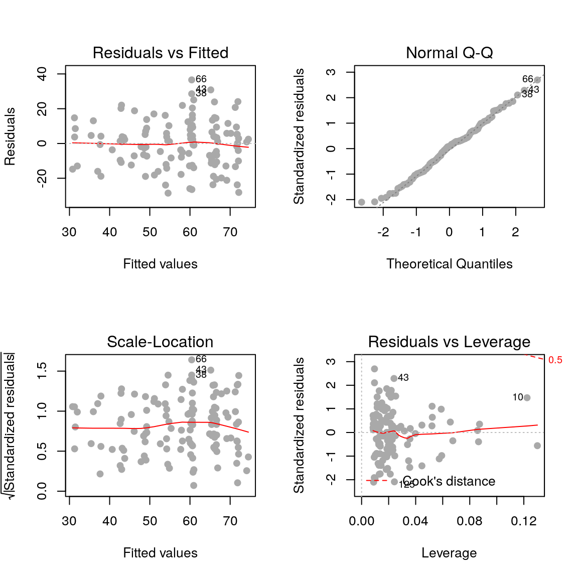
par(mfrow=c(2, 2))
plot(fit, pch=19, col='darkgrey')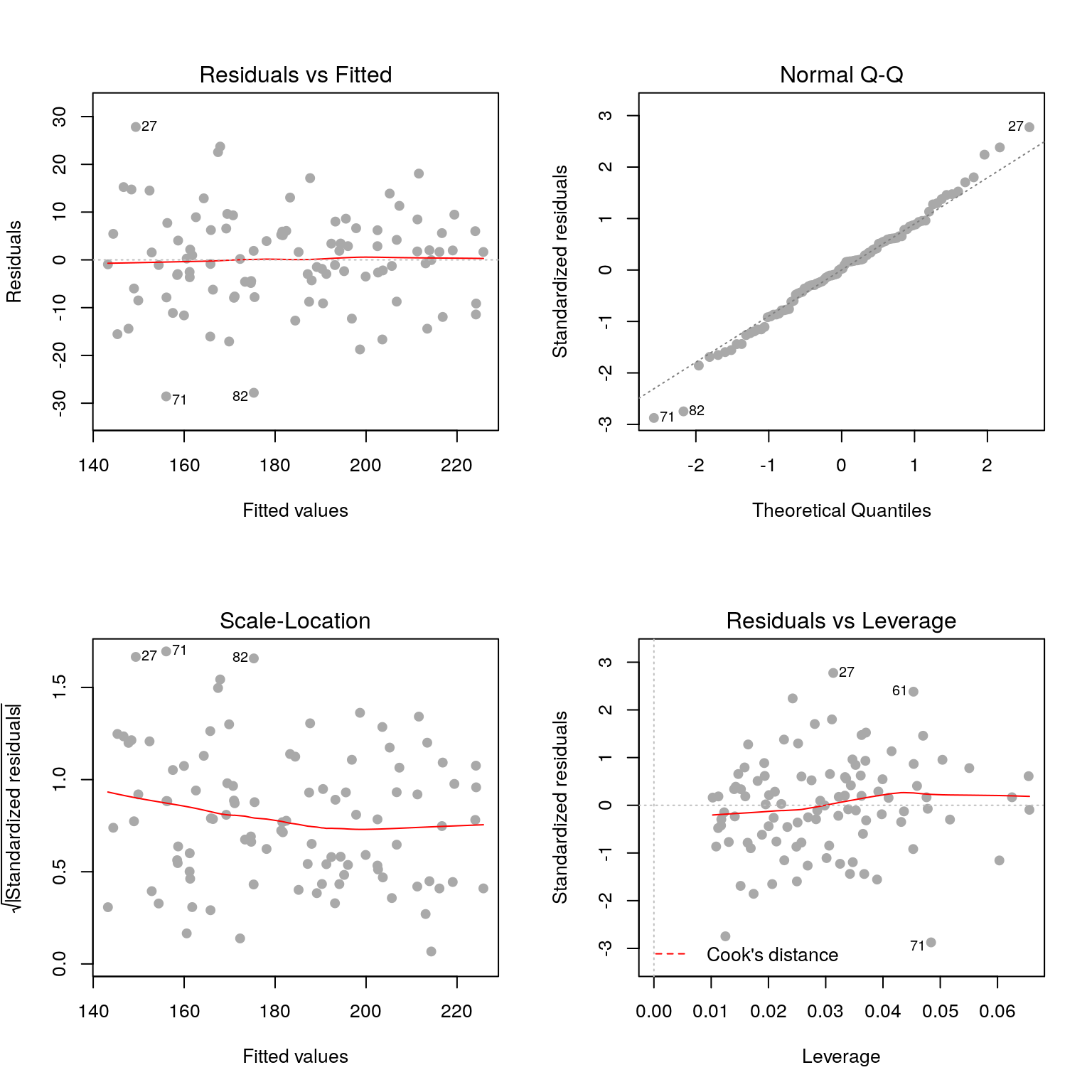

We can extend this framework to any arbitrary large number of explanatory variables. The model is:

\[ \begin{aligned} y_i & = \beta_0 + \beta_1x_{1i} + \ldots + \beta_px_{pi} + \epsilon_i \\ \epsilon_i & \sim \mathcal{N}(0, \sigma^2) \end{aligned} \] Where \(i\) is an index that goes from 1 to \(n\) (the total number of observations) and \(p\) is the total number of explanatory variables. Hopefully it is now clearer why statisticians use Greek letters \(\beta_0, \ldots, \beta_p\), else the equation would be too long to write in English

outcome = intercept + ((gradient outcome vs explanatory variable 1) x (explanatory variable 1)) + ((gradient outcome vs explanatory variable 2) x (explanatory variable 2)) + …)

2.7 Practical 2

We will use the fruitfly dataset (Partridge and Farquhar (1981)) as we did in the previous practical

Task

1. Fit a linear model with lifespan as response variable and thorax length and sleep as explanatory variables
2. Display a summary of the fit, together with the 97% confidence intervals for the estimated parameters
3. What’s the practical significance of the estimated parameters?
4. Show the diagnostic plots for the model, what can you say about the model fit?
5. What is the total variation explained by thorax and sleep?

Solution

fit <- lm(longevity ~ thorax + sleep, ff)
summary(fit)

## 
## Call:
## lm(formula = longevity ~ thorax + sleep, data = ff)
## 
## Residuals:
##     Min      1Q  Median      3Q     Max 
## -28.548 -10.062   1.116   8.787  36.572 
## 
## Coefficients:
##              Estimate Std. Error t value Pr(>|t|)    
## (Intercept) -60.53266   13.07649  -4.629 9.24e-06 ***
## thorax      144.89926   15.85031   9.142 1.68e-15 ***
## sleep        -0.04193    0.07731  -0.542    0.589    
## ---
## Signif. codes:  0 '***' 0.001 '**' 0.01 '*' 0.05 '.' 0.1 ' ' 1
## 
## Residual standard error: 13.64 on 122 degrees of freedom
## Multiple R-squared:  0.4065, Adjusted R-squared:  0.3968 
## F-statistic: 41.79 on 2 and 122 DF,  p-value: 1.502e-14

confint(fit, level=0.97)

##                   1.5 %      98.5 %
## (Intercept) -89.2456056 -31.8197076
## thorax      110.0956304 179.7028839
## sleep        -0.2116944   0.1278351

par(mfrow=c(2, 2))
plot(fit, pch=19, col='darkgrey')

par(mfrow=c(1, 1))

Practical significance of estimated parameters

The intercept parameter (-60.5 days) represents the expected longevity for a fruitfly that has a thorax length of zero and that spends no time sleeping. This is of course biologically implausible, but again acts as a reminder that the linearity assumption is not necessarily true outside the range of the observed data

The thorax parameter (145 days/mm) is the expected increase in longevity for every 1mm increase in thorax. A 1mm increase in thorax length is huge and so for ease of interpretation we can instead state it as 14.5 days per 0.1mm increase in thorax length. The confidence intervals around this parameter is relatively narrow and always positive, suggesting that having a longer thorax is associated with an increased lifespan.

The sleep parameter (-0.0419days/%) is the expected increase in longevity for every 1% increase in sleep. This parameter has a standard error which is comparable to the parameter estimate itself, suggesting a huge uncertainty around this estimate. This is reflected in the 97% confidence intervals which spans from a negative to a positive value. It is therefore unlikely that sleep is associated with longevity.

Model fit

All of the diagnostic plots look sensible, suggesting that our model assumptions are satisfied.

Explained variation

The \(R^2\) statistic (also known as the coefficient of determination) is the proportion of the total variation that is explained by the regression. Which in this case is 40.7%. This is essentially the same as the previous model which only contained thorax, suggesting that sleep is not an important predictor of longevity.

2.8 Categorical explanatory variables

So far we have only considered continuous explanatory variables. How do we include categorical explanatory variables? Let’s go back to our height vs weight toy example and consider sex as an additional categorical variable. Let us simulate some data.

set.seed(101)

## no. of observations
N <- 50 

## hypothetical weights in kg
weightMale <- runif(n=N, min=60, max=100) 

 ## hypothetical weights in kg
weightFemale <- runif(n=N, min=60, max=100)

## hypothetical heights in cm
heightMale <- 2.2*weightMale + rnorm(n=N, mean=0, sd=10) + 40  

## hypothetical heights in cm
heightFemale <- 2.2*weightFemale + rnorm(n=N, mean=0, sd=10) + 2 
height <- c(heightMale, heightFemale)
weight <- c(weightMale, weightFemale)
sex <- c(rep('Male', N), rep('Female', N))

## Store in data frame
df <- data.frame(weight=weight, sex=sex, height=height)

## Plot
plot(height ~ weight, data=df, 
     pch=19, xlab='Weight (kg)', 
     ylab='Height (cm)', col='grey')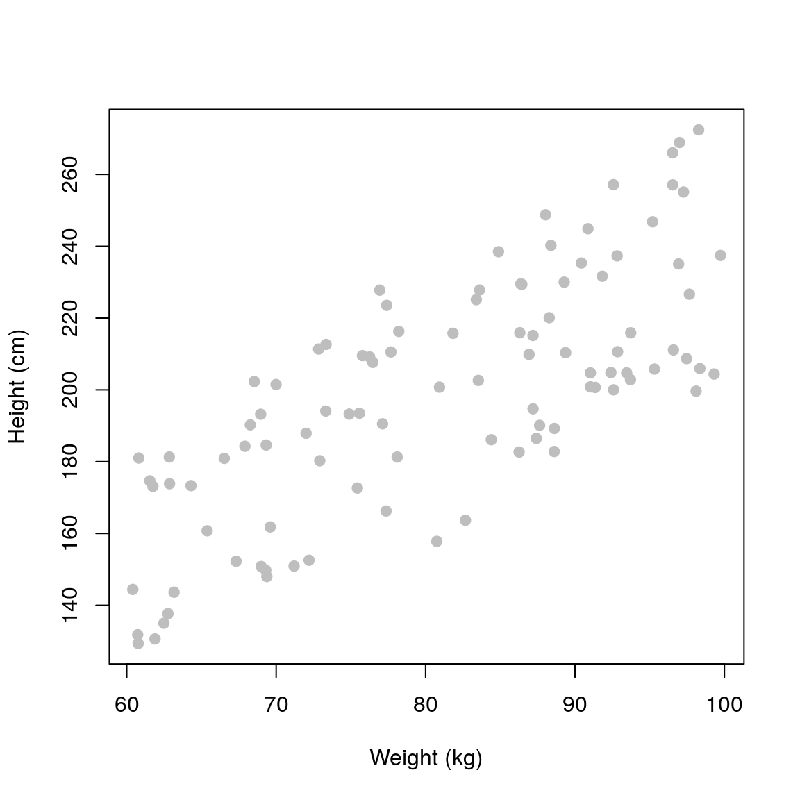

ggplot(df) + 
    geom_point(
        aes(x = weight, y = height)) +
    xlab("Weight (kg)") + 
    ylab("Height (cm)")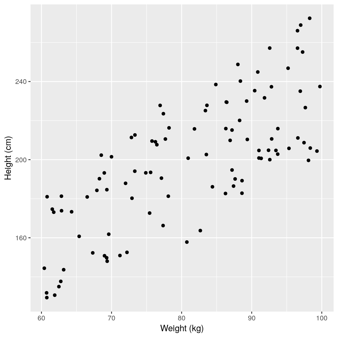

Data looks similar as before, albeit with a larger variation. We can fit a model as we have done before and assess the relationship between height and weight.

## Linear model fit
fit <- lm(height ~ weight, data=df)

## predictions
newdata <- data.frame(
    weight = seq(min(df$weight), 
        max(df$weight), length.out = 50))
newdata$height <- predict(fit, newdata)

## Plot model fit
plot(height ~ weight, data = df, 
     pch=19, xlab='Weight (kg)', 
     ylab='Height (cm)', col='grey')
lines(height ~ weight, data = newdata, 
     col='black', lwd=3)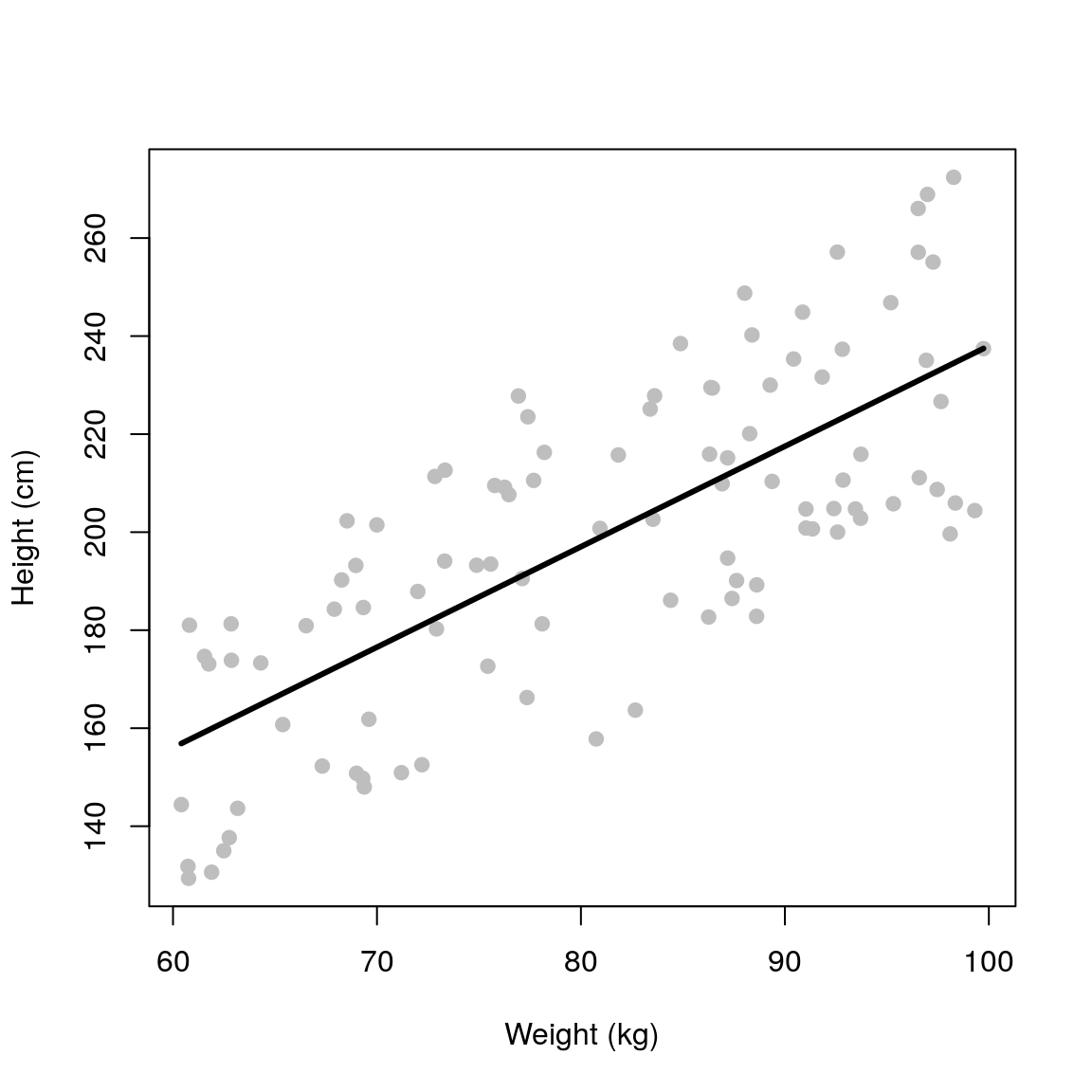

## plot model fit
newdata <- data.frame(
    weight = seq(min(df$weight), 
        max(df$weight), length.out = 50))
newdata <- mutate(newdata, 
    height = predict(fit, newdata))
ggplot(mapping = 
        aes(x = weight, y = height)) + 
    geom_point(data = df) +
    geom_line(data = newdata) +
    xlab("Weight (kg)") + 
    ylab("Height (cm)")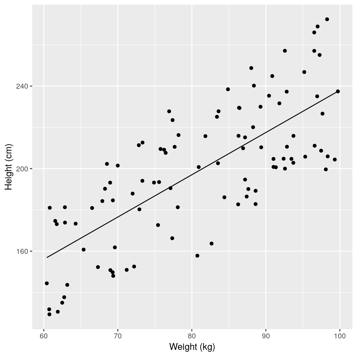

## Print result
summary(fit)

## 
## Call:
## lm(formula = height ~ weight, data = df)
## 
## Residuals:
##     Min      1Q  Median      3Q     Max 
## -40.753 -20.526   2.579  18.889  37.925 
## 
## Coefficients:
##             Estimate Std. Error t value Pr(>|t|)    
## (Intercept)  33.0877    15.2188   2.174   0.0321 *  
## weight        2.0493     0.1859  11.024   <2e-16 ***
## ---
## Signif. codes:  0 '***' 0.001 '**' 0.01 '*' 0.05 '.' 0.1 ' ' 1
## 
## Residual standard error: 22.08 on 98 degrees of freedom
## Multiple R-squared:  0.5536, Adjusted R-squared:  0.549 
## F-statistic: 121.5 on 1 and 98 DF,  p-value: < 2.2e-16

If we colour the data by sex it becomes obvious that this extra variation is due to sex.

plot(height ~ weight, data = df, 
     pch = 19)
points(height ~ weight, 
       pch = 19, 
       data = df[df$sex == "Female", ], 
       col = "green")
points(height ~ weight, 
       pch = 19, 
       data = df[df$sex == "Male", ], 
       col = "blue")
legend(par("usr")[1] * 1.1, 
       par("usr")[4] * 0.9,
       legend = c("Female", "Male"),
       pch = c(19, 19),
       col = c("green", "blue"))

ggplot(df, 
       aes(x = weight, y = height, 
           colour = sex)) +
    geom_point()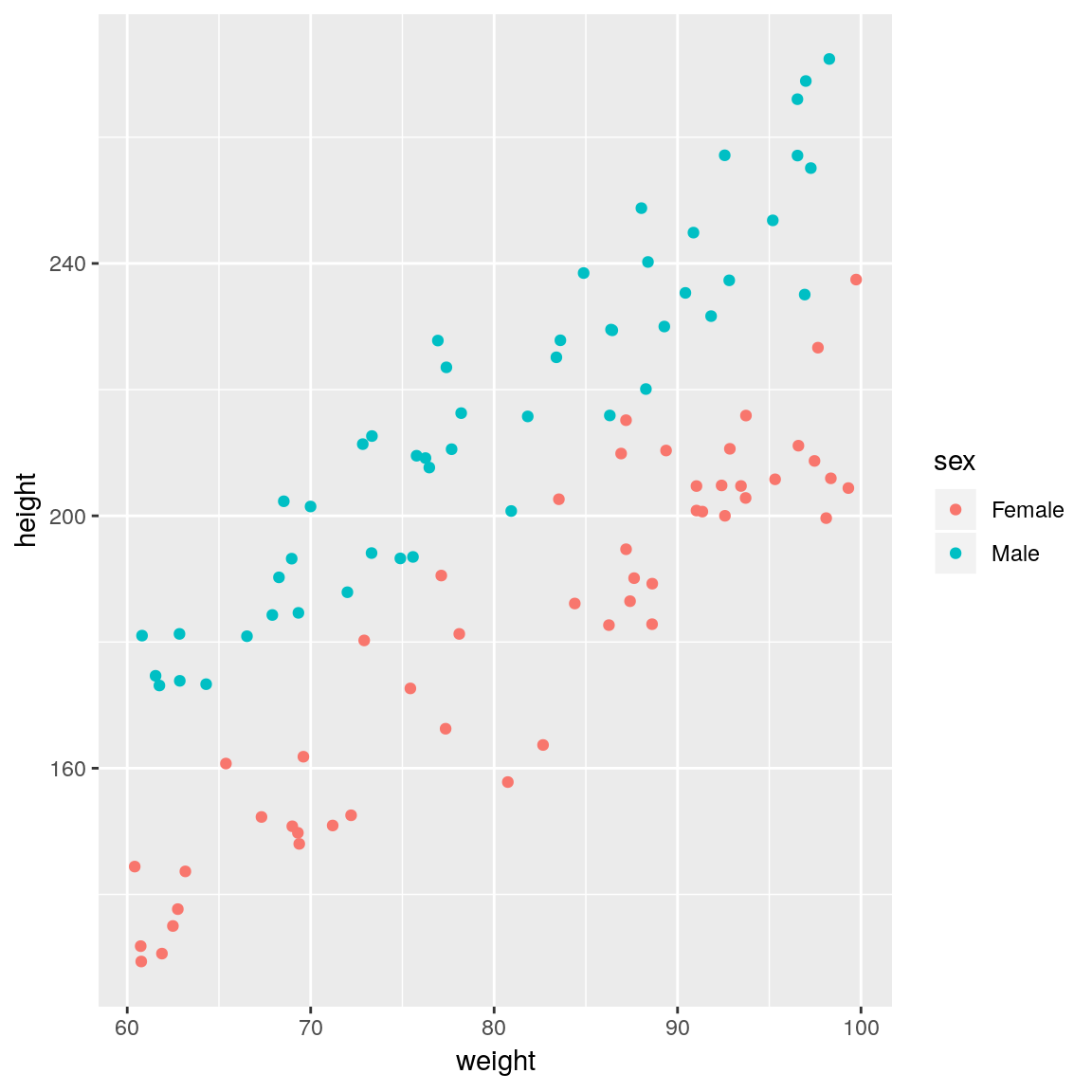

sex is an important covariate and should therefore be added to the model. That is, we need a model that has different regression lines for each sex. The syntax for the R formula remains exactly the same response ~ explanatory_1 + ... + explanatory_p, but behind the scenes categorical variables are treated differently to continuous variables.

To cope with categorical variables (known as factors in R’s lingo), we introduce a dummy variable.

\[ S_i = \left\{\begin{array}{ll} 1 & \mbox{if $i$ is male},\\ 0 & \mbox{otherwise} \end{array} \right. \]

Here, female is known as the baseline/reference level

The regression is:

\[ y_i = \beta_0 + \beta_1 S_i + \beta_2 x_i + \epsilon_i \] Or in English:

\[ \begin{aligned} \mathrm{height}_i & = \beta_0 + \beta_1\mathrm{sex}_i + \beta_2\mathrm{weight}_i + \epsilon_i \\ \end{aligned} \] Where sex is the dummy variable S_i that can take the value of 0 (female) or 1 (male)

The mean regression lines for male and female now look like this:

• Female (sex=0)

\[ \begin{aligned} \mathrm{height}_i & = \beta_0 + (\beta_1 \times 0) + \beta_2\mathrm{weight}_i\\ \mathrm{height}_i & = \beta_0 + \beta_2\mathrm{weight}_i \end{aligned} \]

• Male (sex=1)

\[ \begin{aligned} \mathrm{height}_i & = \beta_0 + (\beta_1 \times 1) + \beta_2\mathrm{weight}_i\\ \mathrm{height}_i & = (\beta_0 + \beta_1) + \beta_2\mathrm{weight}_i \end{aligned} \] By introducing a dummy variable, we have now simplified the problem into two regression lines, where the intercept is:

• Female: \(\beta_0\)
• Male: \(\beta_0 + \beta_1\)

Whilst the gradient is \(\beta_2\) in both cases.

## Linear model fit
fit <- lm(height ~ sex + weight, data=df)

## Print result
summary(fit)

## 
## Call:
## lm(formula = height ~ sex + weight, data = df)
## 
## Residuals:
##     Min      1Q  Median      3Q     Max 
## -21.106  -6.853  -1.162   6.691  22.111 
## 
## Coefficients:
##             Estimate Std. Error t value Pr(>|t|)    
## (Intercept)   1.8269     7.0411   0.259    0.796    
## sexMale      39.2220     1.9976  19.634   <2e-16 ***
## weight        2.1931     0.0841  26.078   <2e-16 ***
## ---
## Signif. codes:  0 '***' 0.001 '**' 0.01 '*' 0.05 '.' 0.1 ' ' 1
## 
## Residual standard error: 9.95 on 97 degrees of freedom
## Multiple R-squared:  0.9103, Adjusted R-squared:  0.9084 
## F-statistic: 491.9 on 2 and 97 DF,  p-value: < 2.2e-16

The sexMale coefficient is \(\beta_1\) in the equations above and it represents the difference in intercept between males and females (remember that the gradient is the same for both sexes). Thus for the same weight, men on average will be sexMale=39.2 cm taller than females.

To plot the fitted lines, we can use a similar trick using predict() as before. This time we need to produce predictions using all relevant combinations of explanatory variables: weight and sex in this case. A useful function to do this is expand.grid():

## create dataset to predict to
newdata <- expand.grid(
    weight = seq(min(df$weight), 
        max(df$weight), length.out = 50),
    sex = c("Female", "Male"))

## generate predictions
newdata <- cbind(newdata, 
    height = predict(fit, newdata))

## plot fitted lines against the data
plot(height ~ weight, data = df, 
    pch = 19)
points(height ~ weight, 
    pch = 19, 
    data = df[df$sex == "Female", ], 
    col = "green")
points(height ~ weight, 
    pch = 19, 
    data = df[df$sex == "Male", ], 
    col = "blue")
lines(height ~ weight, 
    data = newdata[
        newdata$sex == "Female", ], 
    col = "green")
lines(height ~ weight, 
    data = newdata[
        newdata$sex == "Male", ], 
    col = "blue")
legend(par("usr")[1] * 1.1, 
    par("usr")[4] * 0.9,
    legend = c("Female", "Male"),
    pch = c(19, 19),
    col = c("green", "blue"))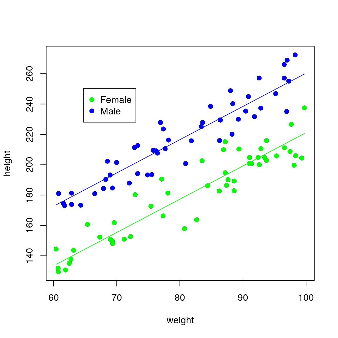

## create dataset to predict to
newdata <- expand.grid(
    weight = seq(min(df$weight), 
        max(df$weight), length.out = 50),
    sex = c("Female", "Male"))

## generate predictions
newdata <- mutate(newdata, 
    height = predict(fit, newdata))

## plot fitted lines against the data
ggplot(mapping = 
        aes(x = weight, y = height, 
            colour = sex)) +
    geom_point(data = df) +
    geom_line(data = newdata)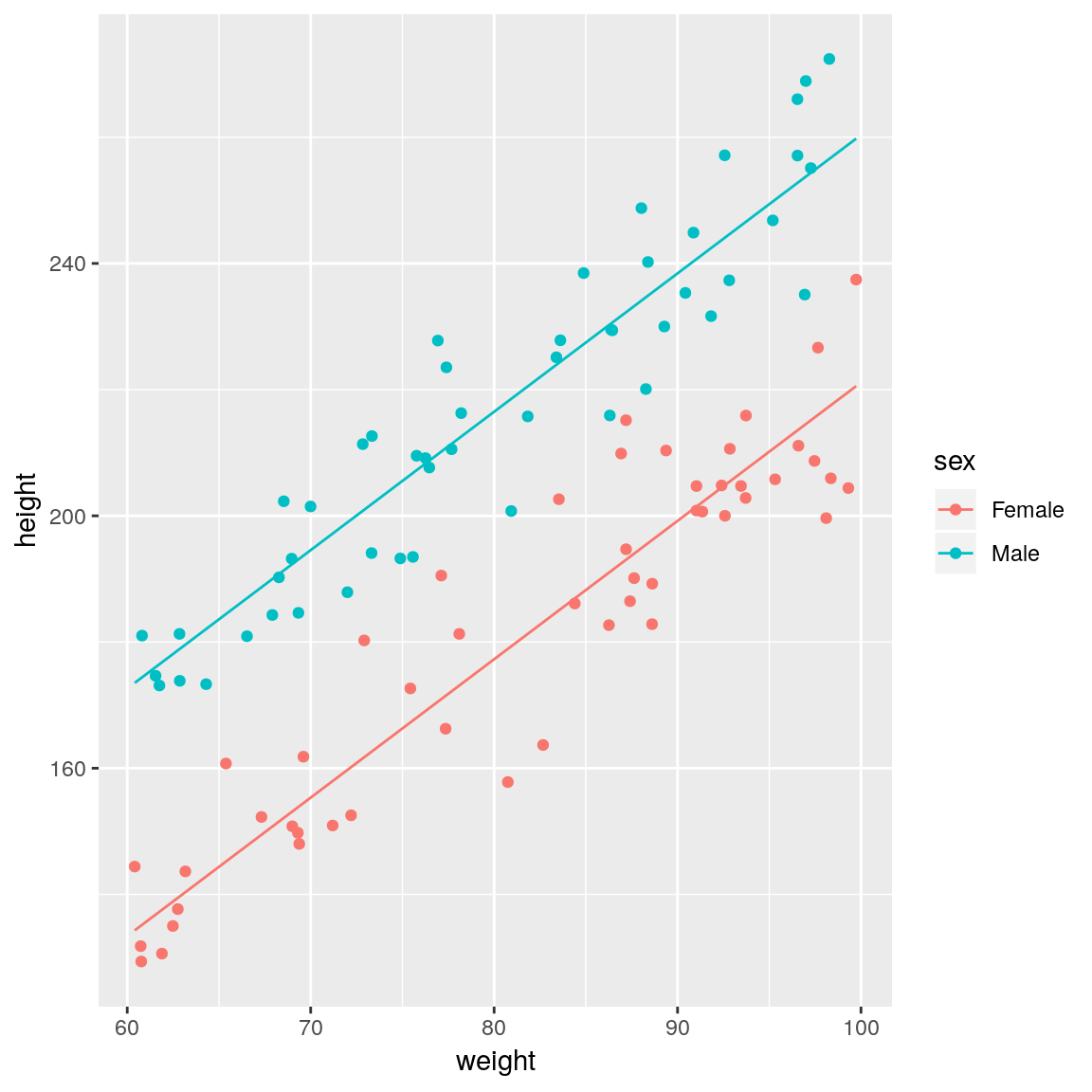

Task

Add 97% confidence intervals to the fitted lines plots above.

Solution

## create dataset to predict to
newdata <- expand.grid(
  weight = seq(min(df$weight), 
    max(df$weight), length.out = 50),
  sex = c("Female", "Male"))

## generate predictions
newdata <- cbind(newdata, 
  predict(fit, newdata, level = 0.97,
    interval = "confidence"))
newdata$height <- newdata$fit
newdata$fit <- NULL

## plot fitted lines against the data
plot(height ~ weight, data = df, pch = 19)
points(height ~ weight, 
  pch = 19, col = "green",
  data = df[df$sex == "Female", ])
points(height ~ weight, 
  pch = 19, col = "blue",
  data = df[df$sex == "Male", ])
lines(height ~ weight, col = "green",
  data = newdata[newdata$sex == "Female", ])
lines(height ~ weight, col = "blue", 
  data = newdata[newdata$sex == "Male", ])
lines(lwr ~ weight, 
  data = newdata[newdata$sex == "Female", ], 
  col = "green", lty = 2)
lines(lwr ~ weight, 
  data = newdata[newdata$sex == "Male", ], 
  col = "blue", lty = 2)
lines(upr ~ weight, 
  data = newdata[newdata$sex == "Female", ], 
  col = "green", lty = 2)
lines(upr ~ weight, 
  data = newdata[newdata$sex == "Male", ], 
  col = "blue", lty = 2)
legend(par("usr")[1]*1.1, par("usr")[4]*0.9, 
  pch = c(19, 19), col = c("green", "blue"),
  legend = c("Female", "Male"))

## create dataset to predict to
newdata <- expand.grid(
    weight = seq(min(df$weight), 
        max(df$weight), length.out = 50),
    sex = c("Female", "Male"))

## generate predictions
newdata <- cbind(newdata, 
    predict(fit, newdata, 
        interval = "confidence", 
        level = 0.97)) %>%
    rename(height = fit)

## plot fitted lines against the data
ggplot(mapping = aes(x = weight)) +
    geom_point(aes(y = height, colour = sex), 
        data = df) +
    geom_line(aes(y = height, colour = sex), 
        data = newdata) +
    geom_ribbon(aes(ymin = lwr, ymax = upr, 
        fill = sex), data = newdata, 
        alpha = 0.5)

Task

Compare the total variation explained by the model with just weight to the one which considers weight and sex. What gives rise to this difference?

Solution

By omitting sex from our model, we have no other alternatives but to treat this extra variation as noise, \(\epsilon_i \sim \mathcal{N}(0, \sigma^2)\). The unexplained variation (\(\sigma^2\)) is due to observation noise and sex. Once we put sex into our model, it will “soak” up the variation that is due to sex which improves our model considerably. The unexplained variation (\(\sigma^2\)) is now only due to the observation error (and other factors that we might be omitting).

Note the baseline/reference level in R is automatically taken to be the first factor level.

levels(df$sex)

## [1] "Female" "Male"

We can change this by re-ordering the levels if we wanted to.

df$sex <- factor(df$sex, levels = c('Male', 'Female'))

## Linear model fit
fit <- lm(height ~ sex + weight, data=df)

## Print result
summary(fit)

## 
## Call:
## lm(formula = height ~ sex + weight, data = df)
## 
## Residuals:
##     Min      1Q  Median      3Q     Max 
## -21.106  -6.853  -1.162   6.691  22.111 
## 
## Coefficients:
##             Estimate Std. Error t value Pr(>|t|)    
## (Intercept)  41.0489     6.8707   5.975 3.81e-08 ***
## sexFemale   -39.2220     1.9976 -19.634  < 2e-16 ***
## weight        2.1931     0.0841  26.078  < 2e-16 ***
## ---
## Signif. codes:  0 '***' 0.001 '**' 0.01 '*' 0.05 '.' 0.1 ' ' 1
## 
## Residual standard error: 9.95 on 97 degrees of freedom
## Multiple R-squared:  0.9103, Adjusted R-squared:  0.9084 
## F-statistic: 491.9 on 2 and 97 DF,  p-value: < 2.2e-16

As expected this change simply changes the sign of the \(\beta_1\) parameter, because the dummy variable now takes the value of 0 for male and 1 for female (i.e we switched things around).

2.9 Practical 3

We will use the fruitfly dataset (Partridge and Farquhar (1981)) as we did in the previous practical

Task

1. Fit a linear model with lifespan as response variable and thorax length and type of companion as explanatory variables
2. Display a summary of the fit, together with the 97% confidence intervals for the estimated parameters
3. Why do we get two parameters for type of companion and what do they mean in practice?

Solution

fit <- lm(longevity ~ type + thorax, ff)
summary(fit)

## 
## Call:
## lm(formula = longevity ~ type + thorax, data = ff)
## 
## Residuals:
##     Min      1Q  Median      3Q     Max 
## -27.330  -6.803  -2.531   7.143  29.415 
## 
## Coefficients:
##                 Estimate Std. Error t value Pr(>|t|)    
## (Intercept)      -56.521     11.149  -5.069 1.45e-06 ***
## typeInseminated    3.450      2.759   1.250    0.214    
## typeVirgin       -13.349      2.756  -4.845 3.80e-06 ***
## thorax           143.638     13.064  10.995  < 2e-16 ***
## ---
## Signif. codes:  0 '***' 0.001 '**' 0.01 '*' 0.05 '.' 0.1 ' ' 1
## 
## Residual standard error: 11.21 on 121 degrees of freedom
## Multiple R-squared:  0.6024, Adjusted R-squared:  0.5925 
## F-statistic:  61.1 on 3 and 121 DF,  p-value: < 2.2e-16

confint(fit, level=0.97)

##                      1.5 %     98.5 %
## (Intercept)     -81.005320 -32.037404
## typeInseminated  -2.609106   9.509537
## typeVirgin      -19.400571  -7.298282
## thorax          114.949413 172.326573

The type of companion parameters

In our toy example we introduced one dummy variable because the variable sex only had two factors (male or female). Type of companion has three factors (inseminated, virgin and control), we therefore need two dummy variables as follows:

\[ S_{1i} = \left\{\begin{array}{ll} 1 & \mbox{if $i$ is inseminated},\\ 0 & \mbox{otherwise} \end{array} \right. \]

\[ S_{2i} = \left\{\begin{array}{ll} 1 & \mbox{if $i$ is virgin},\\ 0 & \mbox{otherwise} \end{array} \right. \]

Here, control is the baseline/reference level for type of companion.

    The mean regression line is:

\[ y_i = \beta_0 + \beta_1 S_{1i} + \beta_2 S_{2i} + \beta_3 x_i \]

Or in English:

\[ \begin{aligned} \mathrm{longevity}_i & = \beta_0 + \beta_1\mathrm{inseminated}_i + \beta_2\mathrm{virgin}_i + \beta_3\mathrm{thorax}_i \end{aligned} \]

Where inseminated is a dummy variable that takes the value of 1 (inseminated) or 0 (otherwise) and virgin is another dummy variable that takes the value of 1 (virgin) or 0 (otherwise). For control both dummy variables are zero.

The mean regression lines for the three cases is as follows:

• Control (inseminated=0 and virgin=0)

\[ \begin{aligned} \mathrm{longevity}_i & = \beta_0 + (\beta_1 \times 0) + (\beta_2 \times 0) + \beta_3\mathrm{thorax}_i\\ \mathrm{longevity}_i & = \beta_0 + \beta_3\mathrm{thorax}_i \end{aligned} \]

• Inseminated (inseminated=1 and virgin=0)

\[ \begin{aligned} \mathrm{longevity}_i & = \beta_0 + (\beta_1 \times 1) + (\beta_2 \times 0) + \beta_3\mathrm{thorax}_i\\ \mathrm{longevity}_i & = (\beta_0 + \beta_1) + \beta_3\mathrm{thorax}_i \end{aligned} \]

• Virgin (inseminated=0 and virgin=1)

\[ \begin{aligned} \mathrm{longevity}_i & = \beta_0 + (\beta_1 \times 0) + (\beta_2 \times 1) + \beta_3\mathrm{thorax}_i\\ \mathrm{longevity}_i & = (\beta_0 + \beta_2) + \beta_3\mathrm{thorax}_i \end{aligned} \]

The intercept for these three regression lines is therefore:

• Control: \(\beta_0\) = intercept=-56.5 days
• Inseminated: \(\beta_0 + \beta_1\) = intercept + typeInesminated = -56.5 + 3.45 = -53.1 days
• Virgin: \(\beta_0 + \beta_2\) = intercept + typeVirgin = -56.5 + -13.3 = -69.9 days

The intercepts per se are not a useful measure as they represent the expected longevity of a fruitfly which has a thorax length of zero, which is clearly absurd. What is important is the difference between these intercepts as it represents a vertical shift in the regression line for the three conditions (see plot).

typeInseminated = 3.45 days is the expected increase in longevity for inseminated with respect to control for any thorax length. Similarly, typeVirgin = -13.3 days, is the expected increase in longevity for virgin with respect to control. We can also compute the expected increase in longevity for virgin with respect to inseminated which is typeVirgin - typeInseminated = -13.3 + 3.45 = -16.8 days.

Task

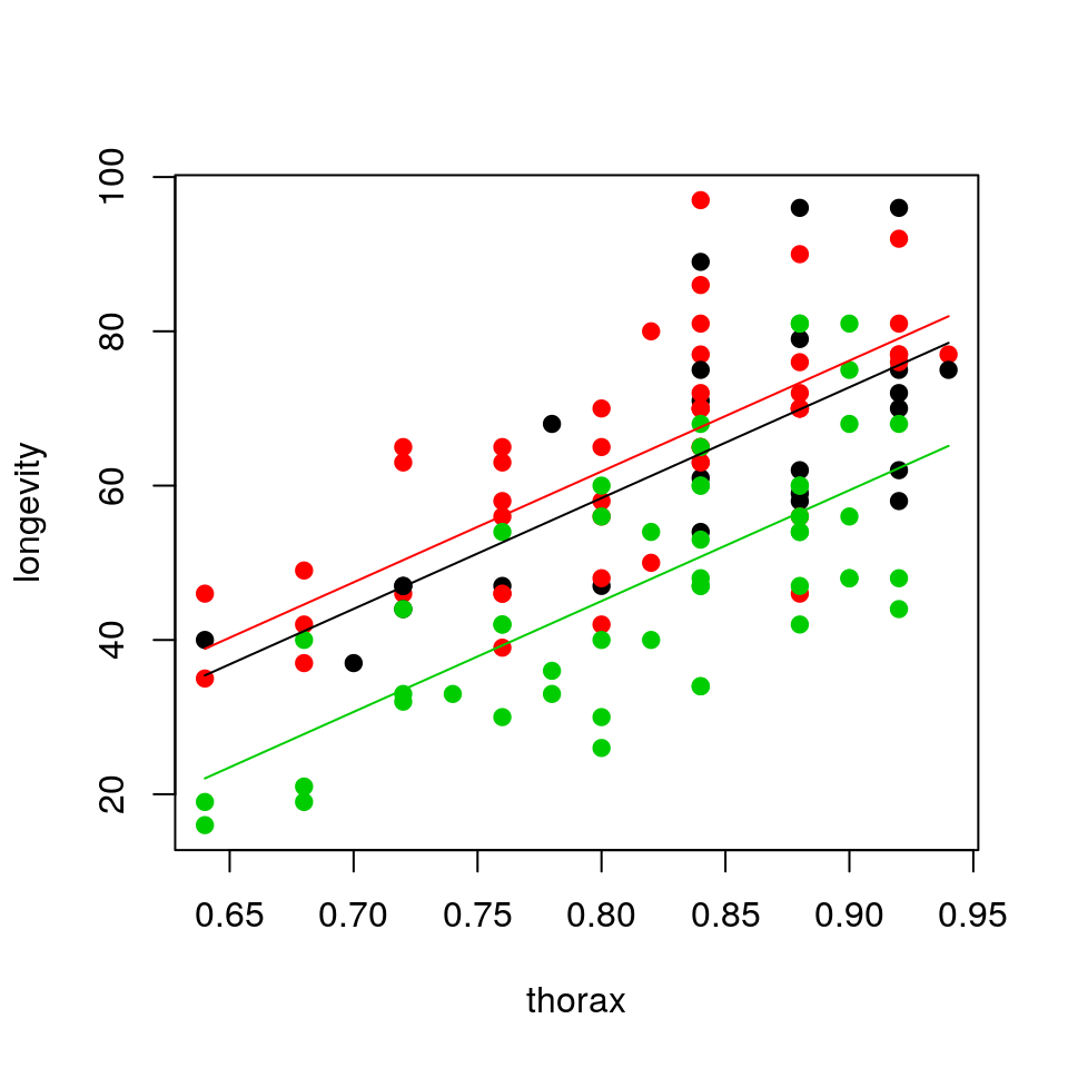
4. Plot the mean regression line for each type of companion together with the observed data.

Solution

newdata <- expand.grid(
    thorax = seq(min(ff$thorax), 
        max(ff$thorax), length.out = 50),
    type = levels(ff$type)
)
newdata <- cbind(newdata, 
    longevity = predict(fit, newdata))
plot(longevity ~ thorax, data = ff, 
     pch = 19, col = as.numeric(ff$type))
for(i in 1:3){
    lines(longevity ~ thorax, 
        data = newdata[newdata$type == 
            levels(ff$type)[i], ], 
        col = i)
}

newdata <- expand.grid(
    thorax = seq(min(ff$thorax), 
        max(ff$thorax), length.out = 50),
    type = levels(ff$type)
)
newdata <- cbind(newdata, 
    longevity = predict(fit, newdata))
ggplot(mapping = aes(x = thorax, y
        = longevity, colour = type)) +
    geom_point(data = ff) +
    geom_line(data = newdata)

Task

5. Show the diagnostic plots for the model, what can you say about the model fit?
6. Compare the total variation explained by this model with the one that only used thorax as a covariate. What can you say about the importance of the type of companion?

Solution

Model fit

par(mfrow=c(2, 2))
plot(fit, pch=19, col='darkgrey')

par(mfrow=c(1, 1))

All of the diagnostic plots look sensible, suggesting that our model assumptions are satisfied.

Explained variation

The \(R^2\) statistic (also known as the coefficient of determination) is the proportion of the total variation that is explained by the regression. Which in this case is 60.2%. This is considerably higher than the 40% achieved with just thorax, suggesting that type of companion is indeed an important covariate and thus should be included in the model.

2.10 Practical issues

The most common issues when trying to fit simple linear regression models is that our response variable is not normal which violates our modelling assumption. There are two things we can do in this case:

1. Variable transformation
   • Can sometimes fix linearity
   • Can sometimes fix non-normality and heteroscedasticity (i.e non-constant variance)
2. Generalised Linear Models (GLMs) to change the error structure (i.e the assumption that residuals need to be normal)

2.11 Summary

Linear regression is a powerful tool:

• It splits the data into signal (trend / mean), and noise (residual error).
• It can cope with multiple variables.
• It can incorporate different types of variable
• It can be used to produce point and interval estimates for the parameters.
• It can be used to assess the importance of variables.

But always check that the model fit is sensible and that the results make sense within the context of the problem at hand. Investigate thoroughly if they do not!!

---

1. this notation is such that we can have any arbitrary large number of explantory variables i.e \(\beta_1\), \(\beta_2\), \(\beta_3\)…etc., without running out of letters in the alphabet!↩

2. weight is our explanatory variable (\(x_i\)) and height the response variable (\(y_i\))↩

3. non-constant variance is known as heteroscedacity↩