3 R Markdown

In the last section we saw that it is possible to generate quick reports directly from R script files. However, this lacks any ability to control the formatting of the output. To this end we can start to think about how to create a simple R Markdown script.

An R Markdown script is usually suffixed with “.Rmd”, but is simply a text file in the same way that standard R scripts are. RStudio offers a useful default template that can be used to initialise a new document. Go to File > New File > R Markdown, and you get an option window that looks like Figure 3.1. In the first instance choose the HTML option and click OK.

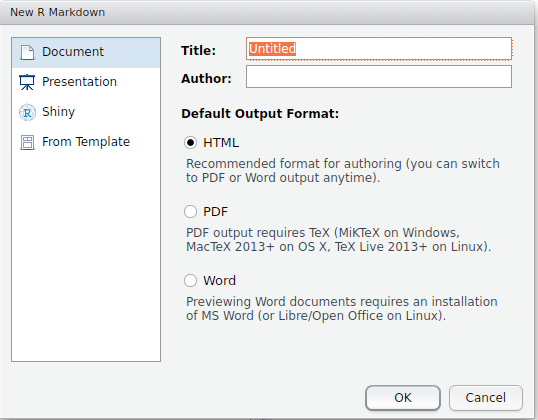
Figure 3.1: R Markdown choices

This creates a new document which looks like Figure 3.2:

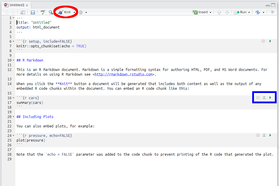
Figure 3.2: R Markdown template

Task

To start with, click the ‘Knit’ button shown by the red circle in the figure above to typeset the document (you will have to save the R Markdown document in your working directory—I called it “test.Rmd”). You can see that it’s produced a HTML document with the code and output weaved together. (As an aside, cars is a dataset provided in the datasets package loaded automatically by R—see ?cars.)

Try compiling to a PDF (if LaTeX is installed), or a Word document by clicking on the arrow next to the ‘Knit’ button and choosing accordingly.

Let’s talk through the different components of the Markdown code.

3.1 YAML

The top section is called the YAML. (This stands for “YAML Ain’t Markup Language”—a recursive acronym of the sort favoured by programmers worldwide.)

## ---
## title: "Untitled"
## output: html_document
## ---

The YAML contains information about the document, and has various options, including: title, author, output, date, toc (table of contents) and so on. The YAML can also be used to provide different options depending on the output document type, for example HTML or PDF.

3.2 Formatting

Formatting in R Markdown is very simple: # denote sections, with subsections denoted by including more hashes (for example ## denotes a second order sub-section and so on). Italics are typeset by enclosing a word or section in single * symbols, for example: *this is in italics* will typeset: this is in italics.

Bold type is written by enclosing a word or section in double * symbols, for example: **this is bold** will typeset: this is bold.

Task

A full list of formatting options can be found in the R Markdown Cheat Sheet. Take a look at this document and familiarise yourself with the options.

3.3 R code chunks

R code chunks can be included by enclosing in backticks ```. For example,

```{r}
summary(cars)
```

will run the code inside the chunk i.e. summary(cars). It will then insert the results from running the code into the output document, so when typeset you will obtain something like:

summary(cars)

##      speed           dist       
##  Min.   : 4.0   Min.   :  2.00  
##  1st Qu.:12.0   1st Qu.: 26.00  
##  Median :15.0   Median : 36.00  
##  Mean   :15.4   Mean   : 42.98  
##  3rd Qu.:19.0   3rd Qu.: 56.00  
##  Max.   :25.0   Max.   :120.00

The chunk can take various options. The first line ```{r}, says that we use the R engine to process the chunk (i.e. that the code inside the chunk should be run in R). The knitr package allows for other languages (such as Python) to be used inside code chunks.

If we want to typeset the code chunk but not run it, we can use the eval option to turn code evaluation off e.g.

```{r, eval = F}
summary(cars)
```

will produce

summary(cars)

(Note: no output chunk.)

Similarly, we can hide the source code but include the outputs by using the echo option e.g.

```{r, echo = F}
summary(cars)
```

will produce

##      speed           dist       
##  Min.   : 4.0   Min.   :  2.00  
##  1st Qu.:12.0   1st Qu.: 26.00  
##  Median :15.0   Median : 36.00  
##  Mean   :15.4   Mean   : 42.98  
##  3rd Qu.:19.0   3rd Qu.: 56.00  
##  Max.   :25.0   Max.   :120.00

(Note: no source code chunk.)

There are various options that can be passed to code chunks, perhaps the most useful being echo and eval (to decide whether source code should be run or not). A full list of options is given in the R Markdown Cheat Sheet.

Task

Have a play with different chunk options using this test document and the R Markdown Cheat Sheet. Familiarise yourselves with the eval and echo options in particular.

3.3.1 Global options

Notice in this template document that there is a chunk at the beginning that looks like

```{r setup, include = FALSE}
knitr::opts_chunk$set(echo = TRUE)
```

The function opts_chunk$set() allows the user to set global options. In this case setting the echo option to be true by default. (Note that options added to individual code chunks override these global options, so I can still set echo = F for particular chunks if required.) Notice also the use of the option include = FALSE to this chunk. This means that the function is run, but neither the source code or outputs are included in the compiled document. This is useful here, since the contents of this chunk relate to the processing of the R Markdown document, and do not play any role in the “analysis”.

Aside: The opts_chunk$set() function is part of the knitr package, and the knitr:: part is just making this explicit. As long as the knitr package is loaded (using library(knitr)), then you do not need to add the knitr:: part. This format can be useful if you want to use specific functions from a package, but without loading the whole library. There are some technicalities around this (RStudio loads the namespace of knitr already—this is not true for all packages), so a more general option would be:
```{r setup, include = FALSE}
library(knitr)
opts_chunk$set(echo = TRUE)
```

This is a useful feature, for example, I often use global options to set figure dimensions (and other useful features, like the tidy option, that tidies code and prevents long lines from overrunning the edge of the code boxes) e.g.

```{r setup, include = FALSE}
knitr::opts_chunk$set(echo = T, eval = T, fig.width = 6, fig.height = 6, 
    tidy.opts = list(width.cutoff = 60), tidy = T)
```

3.3.2 Named chunks

Chunks can also be named. In the example, one chunk looks like:

```{r cars}
summary(cars)
```

Here they have named the chunk cars (the name is the first argument after the r engine indicator, unless we pass named arguments). Naming is useful if we wish to reuse chunks later on, without rewriting all the code. Personally I only name chunks if I wish to reuse them. Chunks must have unique names else knitr will throw an error. If names are not provided, then knitr generates them for you. To reuse earlier named code chunks, one can enclose the name of the required chunk in << >> operators. In the example above, the chunk is named cars, and hence a second chunk

```{r}
<<cars>>
```

will typeset

summary(cars)

##      speed           dist       
##  Min.   : 4.0   Min.   :  2.00  
##  1st Qu.:12.0   1st Qu.: 26.00  
##  Median :15.0   Median : 36.00  
##  Mean   :15.4   Mean   : 42.98  
##  3rd Qu.:19.0   3rd Qu.: 56.00  
##  Max.   :25.0   Max.   :120.00

There is also a facility for including chunks specified in external files, using the read_chunk() function. We will not explore this here, but if you’re interested, a nice example can be found in a ZevRoss blog.

3.3.3 Inline chunks

R Markdown also allows for inline chunks. These are code chunks enclosed in single backtick characters. For example, a line written in R Markdown as,

The mean speed of cars is `r mean(cars$speed)`

then this will typeset as,

The mean speed of cars is 15.4.

Removing the r from the inline chunk will simply typeset the command as a piece of code, but does not evaluate it. Hence,

`mean(cars$speed)`

(note this is enclosed in single backticks `, typesets as

mean(cars$speed).

Task

Have a play with including inline code and typesetting commands using this test document and the R Markdown Cheat Sheet.

RStudio has options that allow you to run code chunks in situ. Note the little green arrow marked in the blue box in Figure 3.2. Clicking this runs each code chunk and returns the output interspersed with the code, allowing for an even more interactive coding environment.

Task

Take the R script you created in the first task of the Reproducibility section. Make a copy of this and save it as an R Markdown file (e.g. if you script was called “ff.R”, copy it to a file called “ff.Rmd”. Edit this file and turn it into a working R Markdown document, with explanations of the analysis interspersed with the code and the output. Make sure you add a title and author to the YAML.

Note: in the solution below I’ve added some further information about the study—for interest’s sake. A separate code file can be found on the workshop website.

Solution


 
---
title: "Sexual activity in fruitflies"
author: TJ McKinley
output: html_document
---

```{r, include = F, purl = F}
knitr::opts_chunk$set(echo = TRUE)
```

# Introduction

A cost of increased reproduction in terms of reduced longevity has been shown for female fruitflies, but not for males. This experiment used a factorial design to assess whether increased sexual activity affected the lifespan of male fruitflies.

The flies used were an outbred stock. Sexual activity was manipulated by supplying individual males with one or eight receptive virgin females per day. The longevity of these males was compared with that of two control types. The first control consisted of two sets of individual males kept with one or eight newly inseminated females. Newly inseminated females will not usually remate for at least two days, and thus served as a control for any effect of competition with the male for food or space. The second control was a set of individual males kept with no females. There were 25 males in each of the five groups, which were treated identically in number of anaesthetizations (using CO2) and provision of fresh food medium.

The data should have the following columns:

* **id**: a ID for each fly in each group (1--25).
* **partners**: number of companions (0, 1 or 8).
* **type**: type of companion (0: newly pregnant female; 1: virgin female; 9: not applicable (when 'partners = 0')).
* **longevity**: lifespan, in days.
* **thorax**: length of thorax, in mm.
* **sleep**: percentage of each day spent sleeping.
* **group**: experimental group (1: control; 2: 1 newly pregnant partner; 3: 8 newly pregnant partners; 4: 1 virgin partner; 5: 8 virgin partners).

Source: [Partridge and Farquhar (1981)](http://www.annualreviews.org/doi/pdf/10.1146/annurev.pu.04.050183.001103)

# Analysis

First we load and summarise the data set:

```{r}
## load the data
ff <- readRDS("ff.rds")

## summarise data
summary(ff)
```

Now plot `thorax` against `group`: 

```{r}
## plot thorax against group
plot(thorax ~ group, data = ff, 
     ylab = "Length of thorax (mm)", 
     xlab = "Experimental group")
```

The plot suggests that thorax length does not seem to vary very much between the experimental groups. Now we plot `longevity` against `group`:

```{r}
## plot longevity against group
plot(longevity ~ group, data = ff,
     ylab = "Longevity (days)", 
     xlab = "Experimental group")
```

The plot suggests that longevity does not seem to vary very much between the experimental groups, with the exception of group 5 (and possibly group 4), which exhibits lower longevity. This is the group where males have 8 virgin sexual partners (i.e. the group that corresponds to a higher degree of sexual reproduction). Finally we plot `longevity` against `thorax`:

```{r}
## plot longevity against thorax
plot(longevity ~ thorax, data = ff, 
     pch = 20, 
     xlab = "Length of thorax (mm)",
     ylab = "Longevity (days)")
```

We can see that there is a strong linear relationship between `thorax` and `longevity`, such that larger flies tend to live longer. On top of this there may be some additional impact of the experimental group, but we will need to investigate further to fully quantify these effects.

3.4 Purling

Note: before you do the next part, make sure you have a backup of your “ff.R” script file; make a copy, use Git or whatever! Just make sure you back it up.

A final point to note is that although it takes a bit of effort to turn an R script file into an R Markdown document, it takes no time to do the reverse. This is because knitr includes a very useful function called purl, that takes the name of an R Markdown file as an argument, extracts all of the code, and creates a new R script file containing just the source code. If your R Markdown file is called “FILE.Rmd”, then by default, purl will create a file called “FILE.R”. There is an output argument to purl that enables you to specify a different file name. (Hence why I said to be careful to make a backup of “ff.R” above).

Note make sure knitr is explicitly loaded using library(knitr) for the next component, or use knitr::purl().

For example, the test document we were playing around with I called “test.Rmd”. Hence,

purl("test.Rmd")

creates a new document in the working directory called “test.R”, which looks like:

## ----setup, include=FALSE------------------------------------------------
knitr::opts_chunk$set(echo = TRUE)

## ----cars----------------------------------------------------------------
summary(cars)

## ----pressure, echo=FALSE------------------------------------------------
plot(pressure)

If you want a different output file name, try something like:

purl("test.Rmd", output = "testscript.R")

Note that R overwrites files by default, so if you run purl multiple times you will overwrite previous versions of the script. So be careful! (Use Git etc.)

Notice that the first chunk is not necessary to include in the R script (it sets knitr options). We can set a purl = F option to an R chunk to tell knitr to exclude the chunk when calling purl. Amending the first chunk in “test.Rmd” to be:

```{r setup, include = FALSE, purl = F}
knitr::opts_chunk$set(echo = T)
```

and then calling purl again, will remove this code chunk from “test.R”.

Task

Take your R Markdown document created in the previous task, and purl it to create a script file (be careful to have a backup of your original script in case you overwrite it).

This makes it easy to share code amongst collaborators. It also means you can write documents with outputs in mind, and work with markdown scripts directly, rather than writing source code and then converting to outputs when finalising analyses. It also forces you to think succinctly, and to write analyses that are readable. Nothing highlights verbose practices more than seeing all the inputs and outputs interspersed.

3.5 Caching

Another feature of R Markdown is the ability to cache results. This means that outputs for chunks that have not changed are stored, and do not have to be rerun every time the document is recompiled. This is really useful if you have several sections of code that take a long time to run. Setting the knitr::opts_chunk$set(cache = T) option will turn caching on. You can turn it on or off from specific chunks by setting a cache = T or cache = F option in the chunk settings. As usual, local chunk options overwrite global ones. The cached files are stored in two folders in the working directory called “FILENAME_cache” and “FILENAME_files”, where FILENAME is the name of your .Rmd file. To remove the cached files, simply delete these two folders.

I generally only do this if some of the code will take a while to run, and I generally delete the cache and rerun from scratch before submitting my final document / code, to ensure reproducibility.

Be warned: If you use un-named chunks, then knitr automatically generates names, hence adding new chunks in will cause the later chunks to be re-run (since the chunk names will change). Also (I think), chunks are only re-run if something changes about the chunk code. Hence if earlier chunks re-create objects used in later chunks, these later chunks will only be re-run if the code changes, not if the object used in the chunk changes. Hence we must be a bit wary when using caching.

3.6 Mathematical equations

R Markdown also allows for the use of mathematical equations through the use of LaTeX commands. For example, the inline code $\int_0^5 x^2 dx$ will typeset as: $\int_0^5 x^2 dx$. Similarly, display style code can be included by enclosing in double $ statements, so the code $$\int_0^5 x^2 dx$$ will typeset as: \[\int_0^5 x^2 dx\].

For guidance, please see a great LaTeX tutorial by Andy Roberts at http://www.andy-roberts.net/writing/latex. Another useful site is DeTeXify, which allows you to hand-draw a symbol and it will find the correct LaTeX term for you!

Task

Write a function that calculates the cumulative distribution function, $P(X \leq x)$, for a Poisson random variable evaluated at some value $x$. Write a short R Markdown document that explains the function, including the mathematical detail using LaTeX equations. Include a plot of the CDF for a Poisson random variable with rate $\lambda = 10$ (for $x \leq 20$).

A solution file is given on the workshop website, or the code can be found below.

3.7 Presentations

You can even write presentations in R Markdown. For example, to write a simple presentation based on Google’s IO theme, you can follow a tutorial here. A Javascipt library I particularly like is reveal.js, which can be implemented in R Markdown easily here. These produce HTML presentations that can be viewed in a web browser. If you want a more traditional approach, you can even use LaTeX’s beamer class to produce PDF slides, as done here.

Task

Write a simple presentation that highlights the key points from your fruitfly analysis you conducted earlier.