3 Fundamentals of R
3.1 Variables in R
R makes use of symbolic variables, i.e. words or letters that can be used to represent or store other values or objects. We will use the assignment operator <- to ‘assign’ a value (or object) to a given word (or letter). Run the following commands to see how this works (don’t worry about the comments, these are for your understanding):
## [1] 5## [1] "Hello There"## we can re-assign variables
y <- sqrt(10)
## or assign a variable in terms
## of other variables
ziggy <- x + y
## print variable "ziggy"
ziggy## [1] 8.162278You will notice that as we create each of these variables, they begin to appear in the environment pane in the top right-hand side of the RStudio window. This shows the current R workspace, which is a collection of objects that R stores in memory. We can remove objects from the workspace using the rm() function e.g.
Notice that x and y have now disappeared from the workspace. The variable ziggy still contains the correct answer though (these are not relative objects, such as the macros assigned in a program like Excel).
## [1] 8.162278Another way of visualising the working directory is to use the ls() function, which lists all objects currently in the workspace e.g.
## [1] "ziggy"Names of variables can be chosen quite freely in R. They can be built from letters, digits and other characters, such as
_. They can’t, however, start with a digit or a.followed by a digit. Names are case sensitive and soheightis a different variable fromHeight. Try to choose informative variable names where possible (heightis more informative thanxwhen talking about heights for example).
Try to use avoid spaces between words in your variable names. Underscores are much safer2. Try to avoid using long words (since you will have to type them out each time you want to access the corresponding elements—although RStudio does have autocomplete functionality). Often I will try to convert as much to lower case as possible. If you do need to include multiple words try to use an underscore
_(e.g.child_heights), or some people prefer to use something like CamelCase (e.g.childHeightsorChildHeights). Use whatever you prefer but try to be consistent.
3.2 Functions in R
Next we need to understand how to do more complicated things in R. For this we need functions. This section illustrates how R’s inbuilt functions work. Most commands that are used in R require the use of functions. These are very similar to mathematical functions (such as log(x)), in that they require both the name of the function (i.e. log) and some arguments (i.e. x). However a lot of functions in R have multiple arguments which can be of completely different types.
The format is that a function name is followed by a set of parentheses containing the arguments. For example, if we type seq(0, 3, 0.5), the function name is seq and the specified arguments are 0, 3 and 0.5. seq() is an inbuilt R function that generates sequences of numbers, and we’re going to continue to use it to illustrate how functions work. Try typing in the command:
## [1] 0.0 0.5 1.0 1.5 2.0 2.5 3.0You can see that this function produces a sequence that starts at 0, ends at 3 and has steps of 0.5. Spaces before the parentheses or between the arguments are not important when writing functions so seq(0,3,0.5) will work just as well as seq (0, 3, 0.5). However, as stated earlier, I think spaces in sensible places can make the code much more legible i.e. seq(0, 3, 0.5) is better than either of the above options.
All functions in R have defaults for the majority of their arguments (some functions have dozens of arguments, and having default values avoids you having to specify them all every time you use the function). For example, the seq() function has the following four main arguments (in this order):
| Argument | Description |
|---|---|
from, to |
the starting and (maximal) end values of the sequence. Of length 1 unless just from is supplied as an unnamed argument. |
by |
number: increment of the sequence. |
length.out |
desired length of the sequence. A non-negative number, which for seq and seq.int will be rounded up if fractional. |
along.with |
take the length from the length of this argument. |
When we write seq(0, 3, 0.5) R assumes that the first argument corresponds to from, the second argument corresponds to to and the third argument corresponds to by. This is known as positional matching. This means that seq(0, 3, 0.5) will produce a vector consisting of the sequence of numbers starting at 0, ending at 3 by adding 0.5 each time. If we write seq(10, 0, 0.5), then R will attempt to create a sequence starting at 10, ending at 0 by adding 0.5 each time.
seq(10, 0, 0.5). R returns an error. Why?
The other type of matching is called named matching and this would allow you to write seq(from = 0, to = 3, by = 0.5) or seq(to = 3, from = 0, by = 0.5) as equivalent function commands (i.e. the order of the arguments doesn’t matter if using named matching).
Using named matching also allows us to access the other argument: length.out if we wanted to use it, though you should recognise that you cannot, in general, use all four arguments in this case to specify a vector. Why not?
In fact, this command needs three arguments to work, and it doesn’t matter which three of the four arguments you use. To find out what arguments a function can take and what they mean use the ?FUNCTION syntax (where you replace FUNCTION with whichever function you’re interested in e.g. ?seq or ?atan). This will open the internal R help file for the function. The Help section of this workshop contains detailed information on these help files.
Being able to access these internal help files will be of particular help for all of the statistical functions we will want to use which generally have many arguments.
Use the R function seq() to create the following sequences:
- 2, 4, 6, …, 30.
- A sequence of 14 numbers starting at -2.5 and ending at 15.34.
- A sequence of 7 numbers starting at 0, increasing in increments of 0.04.
- A sequence starting at 101, ending at -20, in decrements of 11.
3.2.1 Nesting functions
A useful feature of R is its ability to nest functions. This can help make the code more concise and avoids the need to create lots of temporary variables. Nonetheless, if used too extensively then this can render code difficult to interpret, so a balance is necessary. For example,
## [1] 23.62434This is a simple nested function, since sqrt(10) produces a single number, which is then used as an argument to the exp() function. Mathematically, this gives \(e^{\sqrt{10}}\). We could have also done this in two steps, but this would have involved creating a temporary variable to store the result of the sum:
## [1] 23.62434To understand nested functions, think about evaluating the inner functions first, seeing what they output and then how that slots into the next function. We will see an example of this later.
3.3 Help files
It is a requirement of R packages that any function made available to an end user as part of a package must be documented in a help file. As such, the ? command is simply a way to get more information on any given function.
For example, if you wanted to know more about how to use the hist function (this function is used for plotting histograms), then you could type:
?histThis will produce something like Figure 3.1 to appear in the in the bottom-right pane.
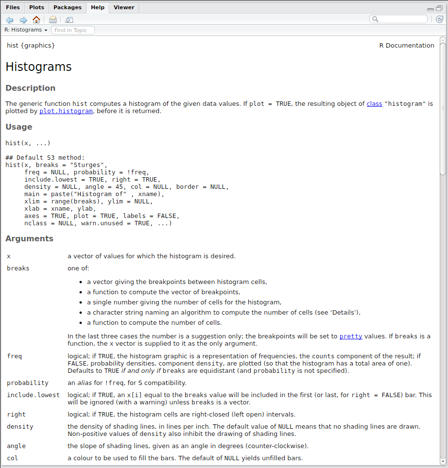
Figure 3.1: Help file for the hist() function
This new window contains all of the information you need to understand how to use the hist() function. Although these help files can seem daunting (and not particularly helpful) at first, once you get used to them they will provide the route for your continued exploration of R. Help files provide all of the details that the author of the command saw fit to include. They all aim to be comprehensive but some authors assume that you are more
familiar with what’s going on than others. Most help files will have the following sections:
| Section | Description |
|---|---|
| Usage: | This will show you the minimum required arguments and also what the default value are for each of the optional arguments. In this case only x is a required argument and all of the others are optional. |
| Arguments: | This gives an explanation of what each argument does and what sort of data type it should be. In this case the argument x needs to be a numerical vector. |
| Details: | This section tells you what the function should do along with any subtleties in its usage or clarifications. |
| Value: | This tells you what actually happens when you run the function and specifically what sort of R object the function produces. In this case it produces a special histogram object (which is actually just a normal list with certain specific components). |
| References: | This gives you some selected text books that the author feels explains the theory behind the function in greater detail. |
| See Also: | This should be a list of other R commands that are related to the current function. They might be of more use to you, or their help files might be better written and clarify what you’re trying to do. |
| Examples: | This should be a set of R commands that you can copy-and-paste into either a script file or the console pane. These should give you a practical example of how to use the function in several different settings. |
If you’re really stuck, there is an international community of R users who regularly post questions and answers on advanced topics. In the Help menu, choose ‘search r-project.org’ and work through the search pages. Beware though, these are busy people who will often ignore directly emailed requests for help. Ask your resident experts first, before e-mailing the R-search email lists!
I also tend to succeed mostly by Googling the problem. For example, Googling ‘R importing data’ finds me this rather excellent tutorial: http://www.r-tutor.com/r-introduction/data-frame/data-import.
3.4 Objects in R
R defines various types of object (and allows you to define your own if you so wish). We will explore the most common object types below.
3.4.1 Vectors
Vectors are fundamental R objects. In fact, we have already seen them at work in earlier examples. For instance, notice that if we type the number 10 into the command prompt, the output when R prints this to the screen is prefixed with a [1]:
## [1] 10This shows that the output is a vector of length 1. The ziggy variable we created earlier is also a vector of length 1:
## [1] 8.162278Note that vectors do not have to be numerical in value e.g.
## [1] "somewords"is also a vector of length 1. R distinguishes between different ‘types’ of vector, with the four main types being:
numericwhere each element is a number (either integer or decimal),characterwhere each element is a word or letter, andfactorwhere each element is a word or letter, but with some additional “grouping” information, andlogicalwhere each element is eitherTRUEorFALSE(equivalently coded asTorF).
In this section we will look at several different commands which produce vectors and then see how we can manipulate these objects in R.
3.4.1.1 Creating vectors
Probably the most common ways of creating vectors are to use the c(), seq() and : commands. Of these, : creates integer sequences, seq() creates structured sequences (only useful for numeric vectors), and c() is short-hand for concatenate, and it binds together all of the elements that you put inside the brackets to make a single vector.
Run the following commands to see how we can create different types of vectors:
## [1] 1 2 3 4 5
## [1] 6 5 4 3 2
Notice that brackets can be important, for example, note the differences below.
## [1] -4 -3 -2 -1  0  1
## [1] -4 -3 -2 -1
The first line above creates an integer sequence from -4 to 1, and the second creates one from -4 to -1. The seq() command we saw earlier, and here are some more examples:
##  [1] 0.0 0.1 0.2 0.3 0.4 0.5 0.6 0.7 0.8 0.9 1.0
## [1] 0.0 0.2 0.4 0.6 0.8 1.0
##  [1] 10.0  9.5  9.0  8.5  8.0  7.5  7.0  6.5  6.0  5.5  5.0
The c() function is very useful for concatenating non-sequential numbers or vectors of other data types e.g.
## [1] 1 3 5 7
## [1]  0.1 -6.0  1.0  0.0
## [1] "bob" "sam" "ted"
Notice that we needed to use double-quotes to signify
charactertypes e.g.c("bob", "sam", "ted"). Note that R does not distinguish between single or double-quotes, soc('bob', 'sam', 'ted')would have worked equally well.
If you forget the quotes (e.g. c(bob, sam, ted)) then R would instead have looked for three objects called bob, sam and ted and tried to concatenate these together. If these objects do not exist, then R will return an error:
## Error in eval(expr, envir, enclos): object 'bob' not foundTo this end, it is worth noting that we can also use c() to concatenate objects that are of the same type together. For example:
## [1] 1.000000 -6.000000 8.162278## [1] 8.162278 3.000000 3.750000 4.500000 5.250000 6.000000(In the example above we have used nested functions to make the code more concise.) If we try to concatenate objects of a different type, R will either return an error, or it will convert one of the objects into the same class as the other. For example,
## [1] "bob"              "sam"              "ted"
## [4] "8.16227766016838"
(Here we use nested c() functions to first create a character vector out of the strings "bob", "sam" and "ted", and then to concatenate this with the object ziggy.) Notice that the concatenated vector is a character vector (notice the double-quotes around "8.16227766016838"), indicating that R has converted the elements of ziggy into characters in order to concatenate them with a character vector.
R will always convert to the most complex object type: so a combination of
characterandnumericvalues will be converted to acharacter.
Notice that R has not changed the value of the object ziggy—if we print ziggy to the screen we can see it is still a numeric vector:
## [1] 8.162278Rather, it created a copy of ziggy which it converted into a character before concatenating. In order to change the value of an object permanently, we need to reassign the object. For example, the function as.character() will convert a numeric vector into a character vector without changing the object e.g.
## [1] "8.16227766016838"## [1] 8.162278To reassign it we can pass the output of the function and overwrite the original object using the assignment operator <- e.g.
## [1] "8.16227766016838"We can see that now the object ziggy has been changed to a character permanently.
Use the various vector creation commands to create the following sequences:
- 1, 2, 3, 4, 5, 6, 7, 8, 9, 10, 11.
- 2, 4, 6, 8, 10, … , 50.
- All of the odd numbers from 17 through to 33.
- The letters of the days of the week (i.e. M, T, W, T, F, S, S).
3.4.1.2 Subsetting and re-arranging vectors
If we only want to get at certain elements of a vector then we need to be able to subset the vector. In R, square brackets [] are used to get subsets of a vector.
IMPORTANT: In R, objects are indexed such that the first element is element
1(unlike C or Python for example, which indexes relative to0). In R the first element ofxisx[1], whereas in Python it would bex[0].Note also that in Python the command
x[-1]would extract the last element of the vectorx, whereas in R the-is used to remove elements; hencex[-1]would remove the first element ofx.
Copy the following commands into your script file and then run them in order to see how this works. Annotate each line using comments to describe what it is doing.
x <- 1:5
x[3]
x[c(2, 3, 4)]
x[1] <- 17
x[-3]
w <- x[-3]
y <- c(1, 5, 2, 4, 7)
y[-c(3, 5)]
y[c(1, 4, 5)]
i <- 1:3
y[i]
z <- c(9, 10, 11)
y[i] <- zCan you work out what the following functions do?
order(y)rev(y)sort(y)
y into decreasing order?
3.4.1.3 Element-wise (or vectorised) operations
R performs most operations on vectors element-wise , meaning that it performs each calculation on each element of a vector or array independently of the other elements. This can make for very fast manipulation of large data sets.
Aside: R is a high-level language, meaning that it is built on low-level languages, in this case C and Fortran. In C, if we wish to apply a function to each element of an array, we need to write a loop. In R there are so-called vectorised functions, that will apply a function to each element of a vector or array. We will cover loops in R later on, but generally they are much slower than the equivalent loops in C or Fortran. The source code for vectorised functions are often written in C or Fortran and hence run much faster than writing a loop in native R code. In addition they make the code more concise. For simple functions the difference in run time is often too small to really notice, but for more complex or large-scale functions the difference in run time can be large. To this end, R also offers various ways of using C code within R functions. But that is beyond the scope of this workshop…
Copy the following commands into your script file and then run them in order to see how this works. Annotate each line using comments to describe what it is doing.
y <- 1:10
y^2
log(y)
exp(y)
x <- c(5, 4, 3, 2, 1, 5, 4, 3, 2, 1)
x + y
x * y
z <- c(-1, 2.2, 10)
z + y
z * yIf you add or multiply vectors of different lengths then R automatically repeats the smaller vector to make it bigger. This generates a warning if the length of the smaller vector is not a divisor of the length of the longer vector. Division and subtraction work in the same way e.g.
## [1] 1 4 3 8 5 12## Warning in c(1:3) * c(1:2): longer object length is not a multiple of
## shorter object length## [1] 1 4 3This is a useful property if the shorter vector is of length 1, in which case R multiplies each element of the longer vector by the scalar e.g.
## [1] 2 4 6You must be very careful with this. I only use this feature when multiplying a vector by a scalar; otherwise I will always generate vectors of the same length, since I think this makes what you are trying to achieve explicit. Hence instead of writing
c(1:6) * c(1:2), I would writec(1:6) * rep(1:2, 3). (I would personally rather that R did not allow elementwise operations on vectors that are of different lengths, but it does, and one should be careful…)
R will also perform matrix multiplication (e.g. dot products) on vectors, and this is described in a later section.
3.4.1.4 Logical vectors and conditional subsetting
Vectors can be created according to logical criteria using the following comparison operators:
| Operator | Definition |
|---|---|
!= |
not equal |
< |
less than |
<= |
less than or equal to |
> |
greater than |
>= |
greater than or equal to |
== |
logical equals |
| |
logical OR |
& |
logical AND |
! |
logical NOT |
Copy the following commands into your script file and then run them in order to see how this works. Annotate each line using comments to describe what it is doing.
x <- 1:10
y <- c(5, 4, 3, 2, 1, 5, 4, 3, 2, 1)
x < 4
x[x < 4]
y[x < 4]
y > 1 & y <= 4
y[y > 1 & y <= 4]
z <- y[y != 3]Finally there are many commands that are specifically aimed at vectors or sets of data. The following is a small selection for reference purposes:
| Function | Description |
|---|---|
length(x) |
returns the length of vector x (i.e. the number of elements in x) |
names(x) |
get or set names of x (i.e. we can give names to the individual elements of x as well as just having them numbered) |
min(x) |
returns the smallest value in x |
max(x) |
returns the largest value in x |
median(x) |
returns the median of x |
range(x) |
returns a vector with the smallest and largest values in x |
sum(x) |
returns the sum of values in x |
mean(x) |
returns the mean of values in x |
sd(x) |
returns the standard deviation of x |
var(x) |
returns the variance of x |
diff(x) |
returns a vector with all of the differences between subsequent values of x. This vector is of length 1 less than the length of x |
summary(x) |
returns different types of summary output depending on the type of variable stored in x |
sum(sqrt(log(seq(1, 10, by = 0.5)))). To help with this, try to write this out in a series of steps and figure out what is returned at each stage of the nesting, and how this is passed to the next function.
3.4.1.5 Factors
We have seen that we can create character vectors. These are collections of strings, but with no further information. For example, if I try to summarise a character vector, R returns no useful information:
##    Length     Class      Mode
##         3 character character
A factor is simply a character vector with some additional “grouping” information attached. For example,
## [1] bob sam ted
## Levels: bob sam ted## bob sam ted
## 1 1 1Now the x object has grouped together all elements of the vector that share the same name (called the levels of the factor), and the summary() function tells us how many entries there are for each level. The levels() function will return the levels of a factor:
## [1] "bob" "sam" "ted"R coerces characters to factors in lexicographical order. If you wish to set specific levels, then you can add a levels argument to the factor() function.
Copy the following commands into your script file and then run them in order to see how this works. Annotate each line using comments to describe what it is doing.
y <- c(5, 4, 3, 2, 10, 5, 4, 3, 2, 1)
factor(y)
factor(y, levels = 1:10)
y <- as.character(c(5, 4, 3, 2, 10, 5, 4, 3, 2, 1))
factor(y)
factor(y, levels = sort(unique(as.numeric(y))))
y <- c("low", "mid", "mid", "high", "low")
factor(y)
factor(y, levels = c("low", "mid", "high"))factor objects are incredibly useful when working with data, since they essentially code up categorical variables, though care must be taken when manipulating them. We explore the use factor objects in more detail in a later section and care must be taken when converting between factors and other types.
3.4.2 Conversions between object types
Before we progress to other objects, we should have a brief aside to talk about conversion between types. So far we have introduced numeric vectors, which store numerical values (note that R makes no distinction between integer, float or double types, like C does). We have also seen character types, which store strings, and factor types that store strings with additional grouping information attached. We have also seen logical types, which simply store TRUE or FALSE values.
It is possible to convert between these different forms, using an as.TYPE() function (where TYPE is replaced with the correct type of interest). For example, we can easily convert numbers to characters:
## [1] 0 1 3 10 0 4## [1] "0" "1" "3" "10" "0" "4"(Notice the double-quotes around the elements of the converted vectors.) They can also easily be converted into factors (if you want to set the levels of the factor specifically, then you can use the factor() function as described earlier):
## [1] 0  1  3  10 0  4
## Levels: 0 1 3 4 10
We can also convert numbers to logical strings, in which case R converts 0 values to FALSE and anything else to TRUE. Hence,
## [1] FALSE TRUE TRUE TRUE FALSE TRUEConversions of logical vectors to numeric vectors results in TRUE values becoming 1 and FALSE values becoming 0.
R can also convert characters to numbers, but only if the conversion makes sense. For example,
## [1] "10" "2" "8"## [1] 10 2 8If the conversion doesn’t make sense, then R will return a missing value (NA) and print a warning:
## Warning: NAs introduced by coercion## [1] 10 2 NAFactors are tricky little blighters! Superficially they can look like numeric types when printed to the screen, but in fact they are named groups, and as such if we convert a factor to a numeric, then R converts according to the level of the factor:
## [1] 10 2  8
## Levels: 10 2 8## [1] 1 2 3Notice that this returns 1, 2, 3 rather than 10, 2, 8.
If a factor holds a numerical value you wish to convert directly, then you must convert the factor to a character first (for which you can often use nested functions to do) e.g.
## [1] 1 2 3## [1] 10 2 8Conversions to character types are straightforward in any case, using as.character(). Conversions of characters or factors to logical types will produce missing values (NA).
3.4.3 Matrices
Matrices are another way of storing data in R. They can be thought of as 2D versions of vectors; a single structured group of numbers or words arranged in both rows and columns. Each element of the matrix is numbered according to the row and column it is in (starting from the top-left corner). The size of the matrix is given as two numbers which specify the number of rows and columns it has. The size is referred to as the dimension of the matrix.
The simplest way of creating a matrix in R is to use the matrix() function.
Copy the following commands into your script file and then run them in order to see how this works. Annotate each line using comments to describe what it is doing.
matrix(1:4, 2, 2)
matrix(1:4, 2, 2, byrow = TRUE)
matrix(0, 3, 4)Like vectors, matrices can also contain character values e.g.
##      [,1] [,2] [,3]
## [1,] "a"  "d"  "g"
## [2,] "b"  "e"  "h"
## [3,] "c"  "f"  "i"
However, all elements must be of the same type. You can have a numeric matrix, or a character matrix, but not a mixture. If you try to specify a mixture then R will convert all entries to the most complex type.
3.4.3.1 Subsetting matrices
Getting access to elements of a matrix follows on naturally from getting access to elements of a vector. In the case of a matrix though you must specify both the row and column of the element that you want, using a format [ROW, COL].
Copy the following commands into your script file and then run them in order to see how this works. Annotate each line using comments to describe what it is doing.
vals <- c(1, 2, 3, 4, 5, 0.5, 2, 6, 0, 1, 1, 0)
mat <- matrix(vals, 4, 3)
mat[2, 3]
mat[1, ]
mat[, 3]
mat[-2, ]
mat[c(1, 3), c(2, 3)]3.4.3.2 Creating matrices
As well as using the matrix() function, we can also create matrices by binding together several vectors (or other matrices). We use two commands here: cbind() and rbind().
Copy the following commands into your script file and then run them in order to see how this works. Annotate each line using comments to describe what it is doing.
x1 <- 1:3
x2 <- c(7, 5, 6)
x3 <- c(12, 19, 25)
cbind(x1, x2, x3)
rbind(x1, x2, x3)Some useful commands for matrices are listed in Table 3.4.
| Function | Example | Description |
|---|---|---|
matrix() |
matrix(0, 3, 4) |
Creates a \((3 \times 4)\) matrix filled with zeros |
dim() |
dim(mat) |
Returns the dimensions of a matrix mat in the form (rows \(\times\) columns) |
t() |
t(mat) |
Transpose a matrix mat |
rownames() |
rownames(mat) |
Returns or sets a vector of row names for a matrix mat |
colnames() |
colnames(mat) |
Returns or sets a vector of column names for a matrix mat |
cbind() |
cbind(v1, v2) |
Binds vectors or matrices together by column |
rbind() |
rbind(v1, v2) |
Binds vectors or matrices together by row |
3.4.3.3 Elementwise operations
Elementwise operations also work similarly to vectors, though even more care must be taken to
Copy the following commands into your script file and then run them in order to see how this works. Annotate each line using comments to describe what it is doing.
x <- matrix(1:9, 3, 3)
x
x * 2
x * c(1:3)3.4.3.4 Matrix multiplication
Another key aspect of matrix manipulation that is required for many algorithms is matrix multiplication. R does this by using the %*% syntax. Note the differences between matrix multiplication and elementwise multiplication:
##      [,1] [,2] [,3]
## [1,]   30   66  102
## [2,]   36   81  126
## [3,]   42   96  150
## [,1] [,2] [,3]
## [1,] 1 16 49
## [2,] 4 25 64
## [3,] 9 36 81Matrix multiplication also works with vectors. In this case the vector will be promoted to either a row or column matrix to make the two arguments conformable. If two vectors are of the same length, it will return the inner (or dot) product (as a matrix). Compare the following (taking note of the comments):
## [1] 1 4 9## [,1]
## [1,] 14## [,1] [,2] [,3]
## [1,] 1 2 3
## [2,] 2 4 6
## [3,] 3 6 9## create new vector
y <- 5:6
## return matrix multiplication of (3 x 1) and (1 x 2) matrix
x %*% t(y)## [,1] [,2]
## [1,] 5 6
## [2,] 10 12
## [3,] 15 18## set up some new matrices
x <- matrix(1:6, 3, 2)
y <- matrix(1:8, 2, 4)
## return matrix multiplication of (3 x 2) and (2 x 4) matrix
x %*% y## [,1] [,2] [,3] [,4]
## [1,] 9 19 29 39
## [2,] 12 26 40 54
## [3,] 15 33 51 693.4.4 Lists
An R list is an object consisting of an ordered collection of objects known as its components (or elements). There is no particular need for the components to be of the same type (unlike vectors), and, for example, a list could consist of a numeric vector, a logical value, a matrix, a complex vector, a character array, and so on.
The following command creates a list object called simpsons, with four components: the first two are character strings, the third is an integer, and the fourth component is a numerical vector. Try creating a list as follows:
The components of a list are always numbered and may always be referred to as such. Thus with simpsons above, its components may be individually referred to as simpsons[[1]], simpsons[[2]], simpsons[[3]] and simpsons[[4]]. Since simpsons[[4]] is a vector, we can access the elements of the vector using the [] notation (i.e. simpsons[[4]][1] is its first element).
The command length(simpsons) gives the number of components it has, in this case four.
The components of lists may also be named (here the names are father, mother, no_children and child_ages) and in this case the component may be referred to either by giving the component name as a character string in place of the number in double square brackets i.e. simpsons[["father"]] (note the double-quotes), or, more conveniently, by giving an expression of the form simpsons$father (note no double-quotes, since father is an object contained within simpsons).
This means that the following will all return the first component of the list simpsons:
## [1] "Homer"## [1] "Homer"## [1] "Homer"The command names(simpsons) will return a vector of the component names of the list simpsons:
## [1] "father" "mother" "no_children" "child_ages"Note the strange double square bracket notation. We can also subset a list using single square brackets, though the returned object is different. For example, typing
## $father
## [1] "Homer"## [1] TRUEreturns a list object, of length 1, where the first element of the list is called father and is a character vector. Using double square brackets returns the character vector itself i.e.
## [1] "Homer"## [1] FALSESometimes we might wish to extract certain components of a list, but keep a list structure, for example
## $father
## [1] "Homer"
##
## $no_children
## [1] 3
produces a list of length 2, containing two components: the first is a character vector called father, and the second is a numeric vector called no_children.
Lists can be useful ways of collecting together a wide range of different bits of information that are all related. R naturally uses lists in a variety of situations but most commonly they are produced as a result of a function call. (In fact most custom classes in R are essentially lists, but with specific methods associated with that class e.g. plot or summary functions for example).
3.4.5 Data frames
A data.frame object is a special type of list where all of the components are in some sense the same size. The simplest form of data.frame consists of a list of vectors all of the same length, but not necessarily of the same type (numeric, character or logical). In this case a data.frame object may be regarded as a matrix with columns for each vector. It can be displayed in a matrix layout, and the data in its rows and columns extracted
using the matrix subsetting notation ([ROWS, COLS]). (However, because it is also a special type of list, we can also extract columns by using the DFNAME$COLNAME notation, where DFNAME is the name of the data.frame of interest, and COLNAME is the name of a specific column. The [[]] notation also works for data.frame objects.)
The important difference (to R at least) between a matrix object and a data.frame object that only contains numeric vectors, is that R thinks of the matrix as a single object, but it thinks of the data.frame as several connected, but distinct objects. (To the user it can be hard to distinguish between objects, and the commands is.matrix(), is.list() and is.data.frame() will return TRUE or FALSE depending on whether an object is a matrix, a list or data.frame respectively.)
data.frames are very important for statistical analysis, as they frequently fit the form of available data. They are so important in fact that a lot of statistical functions actually expect this, and we devote an entire later practical to reading, summarising, plotting and manipulating data.
3.5 Saving outputs
R allows you to save various things, with regards to inputs we can save:
- the full history of all commands used in the current session—via
savehistory(). This creates text files with ‘.Rhistory’ suffixes. - Individual script files (as text files with ‘.R’ suffixes). We’ve already seen these.
With regards to outputs we can save:
- the current R workspace—via
save.image(). This creates a binary file with a ‘.RData’ suffix. This can be reloaded into R using theload()function, and includes all objects in the current workspace. - A selection of objects—via the
save()function. Here we can extract subsets of objects and save them. For example,save(x, y, file = "practical1.RData")will save only the objectsxandyinto a file called “practical1.RData”. Alternatively a character vector of objects can be supplied e.g.save(list = c("x", "y"), file = "practical1.RData")will do the same thing as the previous command. - A single object can be saved using
saveRDS(). This saves into a binary file with a suffix ‘.rds’. This is really useful for saving single objects, often cleaneddata.frameobjects, which can be loaded into R without having to recreate from a ‘.csv’ file for example. For example,saveRDS(x, "x.rds")would save thexobject into a file called “x.rds”. This can be loaded into a new session via thereadRDS()function. Another useful feature is thatreadRDS()can be used to pass the contents of a .rds file directly into an object of your choice e.g.y <- readRDS("x.rds")will create a new object calledy, that contains the contents of the file “x.rds”.
3.6 Reading in data
Most data are stored in e.g. Excel files. Although some packages allow Excel files to be read directly into R, it is (in my opinion) much better practice to save the data as a text file, since this strips out unnecessary formatting and results in smaller file that can be universally used by any end user. Excel also has lots of other problems; see e.g. here.
Aside: You can save Excel spreadsheets as comma-separated text files using e.g. File > Save As > …, then from the ‘Save as type’ options choose ‘CSV (comma separated)’. There is no need to add a suffix, because Excel will automatically add ‘.csv’ to your file name.
.csv files can be read into R directly as data.frame objects, using the read.csv() function.
Note: A .csv file is simply a text file where each element is separated by a comma (the delimiter). This can be easily viewed and manipulated in any text editor (such as Notepad). Many R users prefer to use ‘Text – Tab delimited’ data files. In this case each entry is delimited by a tab. In fact, one can use any delimiter one prefers, but I often prefer commas, which are so common they have their own suffix! If you choose the tab-delimited route, you have to be extra careful about spaces between words in your spreadsheet, and to read the data file into R you should use
read.table()instead ofread.csv()(where you can explicitly specify the delimiter as an argument to the function). This is similarly true if using .csv files: one must be careful not to include entries with commas in them.
Note:
read.csv()might fail if there are any spaces between words within data cells. If this happens, replace all these spaces by underscores_before saving the spreadsheet in Excel.
In fact, it is good practice to store your data in a much simpler way than many people are used to. Generally, try to avoid spaces between words at all in your data, even in column headers. Underscores are much safer. Try to avoid using long words (since you will have to type them out each time you want to access the corresponding elements), and often I will try to convert as much to lower case as possible (since R is case sensitive, so it speeds up your typing).
Download a sample data file: worms.csv. We can load this into R using the read.csv() function, here storing the resulting data.frame as an R object called worms:
If R can’t find the file, check it’s in the working directory, or pass the full path to
read.csv().
##        Field.Name Area Slope Vegetation Soil.pH  Damp Worm.density
## 1     Nashs Field  3.6    11  Grassland     4.1 FALSE            4
## 2  Silwood Bottom  5.1     2     Arable     5.2 FALSE            7
## 3   Nursery Field  2.8     3  Grassland     4.3 FALSE            2
## 4     Rush Meadow  2.4     5     Meadow     4.9  TRUE            5
## 5 Gunness Thicket  3.8     0      Scrub     4.2 FALSE            6
## 6 Oak Mead 3.1 2 Grassland 3.9 FALSE 2## Field.Name Area Slope Vegetation
## Ashurst : 1 Min. :0.800 Min. : 0.00 Arable :3
## Cheapside : 1 1st Qu.:2.175 1st Qu.: 0.75 Grassland:9
## Church Field: 1 Median :3.000 Median : 2.00 Meadow :3
## Farm Wood : 1 Mean :2.990 Mean : 3.50 Orchard :1
## Garden Wood : 1 3rd Qu.:3.725 3rd Qu.: 5.25 Scrub :4
## Gravel Pit : 1 Max. :5.100 Max. :11.00
## (Other) :14
## Soil.pH Damp Worm.density
## Min. :3.500 Mode :logical Min. :0.00
## 1st Qu.:4.100 FALSE:14 1st Qu.:2.00
## Median :4.600 TRUE :6 Median :4.00
## Mean :4.555 Mean :4.35
## 3rd Qu.:5.000 3rd Qu.:6.25
## Max. :5.700 Max. :9.00
## Looking at the data we can see a number of things:
- Since the original data had spaces in the column names, these spaces have been replaced by dots.
- Columns that can be converted into numbers in sensible ways are stored as such (e.g. the
Areacolumn). You can tell this because thesummary()function returns numerical summaries. - Columns that can be converted into logical objects are stored as such (e.g. the
Dampcolumn). - Columns that can’t be easily converted are stored as
factors (e.g. theVegetationcolumn). You can tell this because thesummary()function returns counts of observations in each group.
These defaults can be useful sometimes for finding errors. For example, if a column of numbers contains a typo that prevents an entry from being converted to a number, then the whole column will be read in as a factor(). Thus if you spot this you can often track down the typo and correct it. Please see the section on converting between types for further details on how to manually convert between types.
Important: it is a good idea to always check and read-in data to ensure each column is in the correct format before progressing any further with your analysis. A common error is that often categorical variables are coded as numbers. For example, a data set might contain numbers
0or1to denote e.g. died/survived. In this case R will read the column in as anumeric, when it should be afactor. In this case you would want to manually convert your column to afactorbefore proceeding.
Objects saved as an ‘.rds’ file can be read in and assigned to objects using the readRDS() function e.g.
## save worms data frame as an .rds file
saveRDS(worms, "worms.rds")

## read in as a new object
worms1 <- readRDS("worms.rds")
Here the new worms1 object is identical to the original worms object. I often read in .csv files, clean them up into the correct formats, and then save as an .rds file for further analysis. Since the .rds file stores R objects directly, then reading in the .rds file means I don’t have to do all the cleaning up again.
Alternative approaches can be found in other packages, and indeed a good package is readr, which is part of the tidyverse suite of packages, which we will introduce in the Advanced Visualisation and Data Wrangling tutorials—see here for a useful cheat sheet. Some other options can be found here.
Some people also use dots, e.g.
child.heights, but in general I would avoid this, since dots are often used when working with functions of specific classes such asprint.lm()↩