Introduction

Introduction
These notes are intended as an introduction and guide to using Python for data analysis and research.
As big a part of this workshop as any of the formal aims listed below, is that you should enjoy yourself. Python is a fun language because it is relatively easy to read and tells you all about what you did wrong (or what module was broken) if an error occurs.
With that in mind, have fun, and happy learning!
Structure of this course
The main components of this workshop are these notes and accompanying exercises.
In addition there will be an introductory talk. From there, you’ll be left to work through the material at your own pace with invaluable guidance and advice available from the workshop demonstrators.
Where appropriate, key points will be emphasized via short interjections during the workshop.
Recap: What is Python?
Python is the name of a programming language (created by Dutch programmer Guido Van Rossum as a hobby programming project!), as well as the program, known as an interpreter, that executes scripts (text files) written in that language.
Van Rossum named his new programming language after Monty Python’s Flying Circus (he was reading the published scripts from “Monty Python’s Flying Circus” at the time of developing Python!).
It is common to use Monty Python references in example code. For example, the dummy (aka metasyntactic) variables often used in Python literature are spam and eggs, instead of the traditional foo and bar. As well as this, the official Python documentation often contains various obscure Monty Python references.
Jargon
The program is known as an interpreter because it interprets human readable code into computer readable code and executes it. This is in contrast to compiled programming languages like C, C++, and Java which split this process up into a compile step (conversion of human-readable code into computer code) and a separate execution step, which is what happens when you press on a typical program executable, or run a Java class file using the Java Virtual Machine.
Because of it’s focus on code readability and highly expressive syntax (meaning that programmers can write less code than would be required with languages like C or Java), Python has grown hugely in popularity and is now one of the most popular programming languages in use.
Aims
During this workshop, hopefully you will cover most if not all of the following sections
- Useful Python concepts like
- Comprehensions (e.g.
[ abs(x) for x in y ]) - Context managers (
with) - Generators (
yield)
- Comprehensions (e.g.
- Numerical analysis with Numpy
- Visualizing data with Matplotlib
- Scipy: Additional modules
Optional sections include
- R-like data analysis with Pandas
- Image Processing with Scikit Image (
skimage) & Scipy’s ndimage submodule - Classical User Intefaces with PyQt5
- Web interfaces with Flask
- Scraping data from web resources
- Object Oriented Programming
We will not be delivering hours of lectures on programming constructs and theory, or detailing how every function of every module works.
Printing the notes
For both environmental reasons and to ensure that you have the most up-to-date version, we recommend that you work from the online version of these notes.
A printable, single page version of these notes is available here.
Errata
Please email any typos, mistakes, broken links or other suggestions to j.metz@exeter.ac.uk.
Installing on your own machine
If you want to use Python on your own computer I would recomend using one of the following “distributions” of Python, rather than just the basic Python interpreter.
Amongst other things, these distributions take the pain out of getting started because they include all modules you’re likely to need to get started as well as links to pre-configured consoles that make running Python a breeze.
- Anaconda (Win, MacOS, Linux) : Commercially backed free distribution
- WinPython (Windows Only) : Open-source free distribution
- Linux : Python 2 is preinstalled on older linux distributions; Python 3 should be installed on newer distributions. To install Python 3, simply use your favourite package manager. E.g. on debian based systems (Debian, Ubuntu, Mint), running
sudo apt-get install python3from a terminal will install Python 3. Alternatively use Anaconda.
Note : Be sure to download the Python 3, not 2, and get the correct acrchitecture for your machine (ie 32 or 64 bit).
More (pythonic) Python
You should already be familiar with basic Python including
- Basic data types (numbers, strings)
- Container types like lists and dictionaries (
list,dict) - Controlling program flow with
if-else,for, etc - Reading and writing files
- Defining functions
- Documenting code
- Using modules
If you are unclear on any of these points, please refer back to the introductory notes.
We will now focus on some additional, sometimes Python-specific, concepts. By this I mean that even if you know how to program in C or Fortran, you will possiby not know for example what a list comprehension is!
Less “universally useful” additional Python concepts have been included in the optional “Additional advanced Python” section.
Easier to ask for forgiveness than permission (EAFP): trying
A common programming approach in Python (as opposed to e.g. C) is to try something and catch the exception (i.e. if it fails).
This is as opposed to the approach used in other languages, which is to carefully check all inputs and not expect the exception to happen.
To do this we use a try-except block, for example
# At this point we have a variable called my_var that contains a string
try:
    num = float(my_var)
except Exception:
    # Calling float on my_var failed, it must not be a
    # string representation of a number!
    num = 0
i.e. instead of carefully inspecting the string contained my_var to determine
whether we can convert it to a number, the Pythonic approach is to simply
try and convert it to a number and handle the case that that fails in
an except block.
Note
You can technically write
try:
    ...
except:
    ...
i.e. omit the
Exception, but this is known as bare exception and will catch every possible error. AddingExceptionwill still catch almost all errors; without it, you won’t even be able to (immediately) terminate your script with ctrl-c!It is almost always best to specify exactly which type of exception you are going to try and allow to happen using
try-except.That way, if something else unexpected happens, you will be notified and Python will terminate in the usual (helpful!) way.
Common Standard Library modules: os and sys
We’ve already encountered os and sys in the introductory notes.
However, there are some common uses of os and sys functions that
merit special mention.
File-name operations: os.path
When, generating full file-paths, or extracting file directory locations, we could potentially use simple string manipulation functions.
For example, if we want to determine the folder of the path string
"C:\Some\Directory\Path\my_favourite_file.txt"
we might think to split the string at the backslash character “" and
return all but the last element of the resulting list (and then
put them together again).
However, not only is this tedious, but it is also then platform dependent (Linux and MacOS use forward-slashes instead of back-slashes).
Instead, it is much better to use the os.path submodule to
- create paths from folder names using
os.path.join - determine a (full) filepath’s directory using
os.path.dirnameoros.path.realpath - Split a file at the extension (for generating e.g. output files) using
os.path.splitextamongst many more useful file path manipulation functions.
Getting command-line input using sys.argv
sys.argv is a list of command line arguments (starting with the
script file name) - you can access it’s elements to get command line
inputs.
To test and play with this you can simply add the lines
import sys
print(sys.argv)
to the top of any (or an empty) script, and run the script.
If you follow the script file name by (a space and then) additional words,
you will see these words appear in the terminal output as being contained in
sys.argv.
Exercise : Quick test of sys.argv
Create a new script (exercise_sys_argv.py) and firstly make it print out the arguments it was passed from the command line.
Next have the script try to convert all arguments (after the script filename) into numbers and print out the squares of the numbers. For any input that was not a number, have it print an message letting the user know.
Run your script with several inputs (after the script file name) to confirm it works.
Sys Answer
import sys

print(sys.argv)


def convert_value(value, index):
    """
    Function that try-s to convert input
    to a number, or prints an error message

    Input are the value to convert, and it's index for the error message
    """
    try:
        num = float(value)
        print(num, "squared is", num**2)
    except:
        print("Could not convert value", value, "at", index, "to a number")


for index, val in enumerate(sys.argv[1:]):
    convert_value(val, index-1)
For example, running python exercise_sys_argv.py 3 4 generates
the output
['...exercise_sys_argv.py', '3', '4']
3.0 squared is 9.0
4.0 squared is 16.0
A more complete description of command line inputs is provided in the optional “additional advanced Python” section, for those requiring more information and more advanced command line input options.
String formatting
Another common Python task is creating strings with formatted representations of numbers.
You should already know that the print function is good at printing out a variety of
data types for us.
Internally, it creates string representations of non-string data before printint the final
strings to the terminal.
To control that process, we often perform what is know as string formatting. To create a format string use the following special symbols in the string
"%s"will be substituted by a string"%d"will be substituted by the integer representation of a number"%f"will be substituted by the float representation of a number
We can also specify additional formatting contraints in these special codes. For example to create a fixed length integer representation of a number we might use
print( "%.8d"%99 )
which outputs 00000099 to the terminal; i.e. the .8 part of the code meant : “always make the
number 8 characters long, (appending zeros as necessary).
NOTE: The new way of doing this is to use the format member function;
print("{:08d}".format(99))
though the old way also still works!
For additional format string options in the context of the newer format string method, see the
documentation here.
Comprehensions
Comprehensions are losely speaking shorthand ways to quickly generate lists, dictionaries, or generators (see later) from relatively simple expressions.
Consider a for loop used to generate a list that holds the
squares of another list:
list1 = [10, 20, 30, 40]
list2 = []
for val in list1:
    list2.append( val * val ) # or equivalently val ** 2
The last 3 lines can be neatly replaced using a list comprehension:
list1 = [10, 20, 30, 40]
list2 = [val*val for val in list1]
That’s it! Simple, clean, and easy to understand once you know how.
In words what this means is: “set list2 to : a new list, where the list
items are equal to val*val where val is equal to each item in list list1“.
list2 will then be equal to [100, 400, 900, 1600].
The list comprehension can work with any type of item, e.g.
list3 = ["spam", "and", "eggs"]
list4 = [ thing.capitalize() for thing in list3 ]
would set list4 equal to ["Spam", "And", "Eggs"].
Similarly you can generate a dictionary (nb. dictionaries are created with braces, aka curly brackets) comprehension
words = ['the', 'fast', 'brown', 'fox']
lengths = {word : len(word) for word in words }
(this generates the dictionary
{'the':3, 'fast':4, 'brown':5, 'fox':3} assigned to lengths)
The last example is using tuple syntax (re: tuples are defined using parentheses, aka round brackets),
list1 = [10, 20, 30, 40]
gen   = ( val * val for val in list1)
but the crucial difference is that gen is not a tuple (nor a list). It is a generator object, which we will learn about below.
Adding logic to comprehensions
Comprehensions can also include simple logic, to decide which elements
to include.
For example, if we have a list of files, we might want to filter the files
to only include files that end in a specific extension. This could be done
by adding an if section to the end of the comprehension;
# e.g. file list
file_list = ["file1.txt", "file2.py", "file3.tif", "file4.txt"]
text_files = [f for f in file_list if f.endswith("txt")]
This code would result in the variable text_files holding the list
["file1.txt", "file4.txt"] - i.e. only the strings that ended in “txt”!
Exercise : Reading a file with a comprehension
Create a new script file (“exercise_comprehensions.py”) and add code to load the comma separated value data that we used in the Introductory exercises on loading data ( available here: data_exercise_reading.csv).
After opening the file, you should skip the first row as before, and then load the numerical
data for the second column (“Signal”) directly into a list,
using a list comprehension, not a for-loop.
Then use the built-in function sum (which operates on iterables) to print the sum as well
as len to print the number of elements.
Comprehensions Exercise
You can copy the code from the introductory exercise on file reading, up to the point where you skipped the first line of the file.
After that, you only need to add 1 line to read all the data and convert it into numbers!.
In order to do so, you will need to remember that you can
iterate over a file object (e.g. for line in file_obj1).
Comprehensions Answer
Using e.g.
# Load data from a text (csv) file using a comprehension
# OPTIONALLY use the current script's location as the data folder, if that's where the data
import os
ROOT = os.path.realpath(os.path.dirname(__file__))

fid = open(os.path.join(ROOT, "data_exercise_reading.csv"))
# Skip the first line (ie read it but don't keep the data)
fid.readline()
# Now read just the Signal data
sig = [ int( line.split(',')[1] ) for line in fid]
fid.close()

print("Signal data loaded:")
print("N        = ", len(sig))
print("Sum      = ", sum(sig))
produces
Signal data loaded:
N        =  2000
Sum      =  199152
Context managers : with
A context manager is a construct to allocate a resource when you need it and handle any required cleanup operations when you’re done.
One of the most common examples of where context managers are useful in Python is reading/writting files.
Instead of
fid = open('filename.txt')
for line in fid:
    print(line)
fid.close()
we can write
with open('filename.txt') as fid:
    for line in fid:
        print(line)
Not only do we save a line of code, but we also avoid forgetting to close the file and potentially running into errors if we were to try and open the file again later in the code.
Context managers are also used in situations such as in the threading module
to lock a thread, and can in fact be added to any function or class
using contextlib.
If you’re interested in advanced uses of context managers, see e.g.
- https://jeffknupp.com/blog/2016/03/07/python-with-context-managers/
- http://preshing.com/20110920/the-python-with-statement-by-example/
- https://www.python.org/dev/peps/pep-0343/
Otherwise, other than switching to using with when opening files,
you probably won’t encouter them too often!
Useful built-in global variables : __file__, __name__
I sneakily introduced some built-in global variables during the Introductory workshop material - apologies to those of you who wondered what they were and where they came from!
The reason I used these variables (namely __file__ and __name__),
was to make things easier with respect to accessing the current script’s
file name, and creating a section of code that would only run if the script
was being run as a script (i.e. not being imported to another script),
respectively.
Firstly a note about naming; the built-in variables are named using two
leading and trailing underscores (__), which in Python is the convention
for letting other developers know that they shouldn’t change a variable.
This is because other modules and functions will likely also make use of these variables, so if you change their values, you might break these other modules and functions!
To recap, two commonly used built-in global variables:
__file__: holds the name of the currently executing script__name__: holds the name of the current module (or the value"__main__"if the script is run as a script - making it useful for adding a script-running-only section of code)
A brief overview of Objects in Python: The “why” of member functions
You have already used modules in Python. To recap; a module is a library of related functions which can be imported into a script to access those functions.
Using a module, e.g. the build-in os module to access operating-system
related functionality, is as simple as adding
import os
to the top of your script.
Then, a module function is accessed using the dot (“.”) notation:
os.listdir()
would for example return the directory listing for the current working directory.
However, you have also seen dot notation used when accessing functions that we’ve referred to as member functions. A member function refers to a function that belongs to an object.
For example, the built-in function open returns a file object.
This file object has member functions such as readlines which is
used to read the entire contents the file into a list.
The reason we are talking about objects is to stress the difference
between a module function like os.listdir, and a member function
e.g.
the_best_file = open("experiment99.txt")
data = the_best_file.readlines()
Another example of a member function that we’ve already used is
append, which is a member function of list objects.
E.g. we saw
list_out = []  # Here we create a list object
for val in list_in:
    list_out.append(val*val)    # Here we call the member-function "append"
As long as we are happy that there are modules which are collections of functions, and independently there are objects which roughly speaking “have associated data but also have member functions”, we’re ready to start learning about one of the most important libraries available to researchers, Numpy.
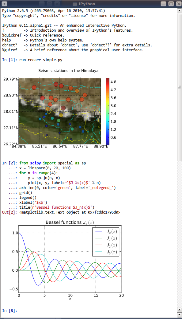
IPython console and Jupyter notebook
Before diving into Numpy in the next section, it’s worth drawing attention to IPython for those of you who haven’t tried it yet.
IPython (for Interactive Python) provides several tools that enhance the Python development experience.
You may have already been using IPython tools (e.g. via Spyder) without being fully aware of it.
The IPython console is an enhanced interactive Python interpreter which imrpoves on the standard interactive interpreter in a number of useful ways:
- syntax highlighting
- tab completion
- Better built-in help system
- Python “magics”, i.e. packaged tools
On Anaconda/WinPython this can be started by opening the IPython Qt Console application, or from a running console by launching ipython3 or jupyter-console.
If Anaconda/WinPython isn’t registered with Windows (i.e. you can’t find it in the Start Menu), you can try using the file explorer to navigate to the Anaconda/WinPython folder (possibly “C:\Anaconda” or “C:\WinPython”) and start the “IPython Qt Console” application.
NOTE The reason that both IPython and Jupyter exist is that IPython was developed first but then (largely in the form of the notebook interface - see below) a more general multi-language (including Julia, Python, R, hence the name, and many others) framework, Jupyter, branched off from the original IPython projct.
Nowadays, Ipython still exists as a Jupyter “kernel”, (amonst many others), and can still be launched via the independent ipython command.
Please note however that while IPython is a great tool it should be just that and resist the temptation to abandon writing your code in scripts!
If you try and write anything vaguely complex in the IPython console, you will quickly find yourself in a pickle when it comes to indentation levels etc, and keeping track of what you did!
In addition variables are all kept in memory making it easy to make mistakes by using a previously defined variable.
The notebook interface
A subequent evolution of the interactive interface provided (first by IPython, now more generally by the Jupyter project) is the notebook.
This is a web interface, which provides cell-based inputs, which Maple or Mathematics users might
find familiar, coupled with inline output, including textual outputs (e.g. from print calls) as
well as inlined plots.
This mix of code and output makes notebooks very attractive for demonstrations, presentations, general teaching, as well as a host of other uses.
However, it should be stressed that while notebooks are very useful for a range of tasks, they are not a good tool for general software development.
There are multiple reasons for this including several major ones
- Preserved state becomes confusing especially when performing out-of-order execution of cells -> leads to repeated use of “restart and run all”, rendering any interactive component much less useful.
- Notebooks tend to promote bad coding practices
- modularisation is harder
- writing tests for code is not straight-forward
- temptation to use non-code cells for documenting code, i.e. not actually documenting code correctly
Exercise : Getting familiar with IPython
For this exercise, instead of writing a script, you’re going to start IPython and get familiar with how to test mini-snippets of code there.
Start the IPython QtConsole, and in the interactive Python session, create variables that hold
- a list holding the numbers
33, 44, 55 - and another that holds a dictionary holding the days of the week (as keys) and the length of the day name (as values)
print your variables to confirm that they hold the required data.
Lastly, type the name of your variable holding the list, then a dot (.) and then press tab.
You should see IPython’s tab completions system pop-up with a list of possible methods. Append the value 66 to the end of the list.
This quick practice of IPython QtConsole operations should get you started in being able to use the console to test small snippets of code!
Exercise : Test out the notebook interface
Launch the jupyter-notebook; a web-page showing the notebook start page should be opened for you.
Practice entering code in cells and evaluating the cells.
In particular, experiment with the %pylab inline magic.
Exercise : Additional notebook-based exercises
If you would like some more exercise based on the content of this page, please download and run the accompanying notebook.
Numerical Analysis with Numpy
Numpy is probably the most significant numerical computing library (module) available for Python.
It is coded in both Python and C (for speed), providing high level access to extremely efficient computational routines.
Basic object of Numpy: The Array
One of the most basic building blocks in the Numpy toolkit is the
Numpy N-dimensional array (ndarray),
which is used for arrays of between 0 and 32
dimensions (0 meaning a “scalar”).
For example,
is a 1d array, aka a vector, of shape (3,), and
is a 2d array of shape (2, 3).
While arrays are similar to standard Python lists (or nested lists) in some ways, arrays are much faster for lots of array operations.
However, arrays generally have to contain objects of the same type in order to benefit from this increased performance, and usually that means numbers.
In contrast, standard Python lists are very versatile in that each list item can be pretty much any Python object (and different to the other elements), but this versatility comes at the cost of reduced speed.
Creating Arrays
ndarrays can be created in a number of ways, most of which directly involve
calling a numpy module function.
From Python objects
Numpy includes a function called array which can be used to
create arrays from numbers, lists of numbers or tuples of numbers.
E.g.
numpy.array([1,2,3])
numpy.array(7)
creates the 1d array [1,2,3], and number (scalar) 7 (albeit as an ndarray!).
Nested lists/tuples produce higher-dimensional arrays:
numpy.array([[1,2], [3,4]])
creates the 2d array
[[1 2]
 [3 4]]
NB: you can create arrays from dicts, lists of strings, and other
data types, but the resulting ndarray will contain those objects
as elements (instead of numbers), and might not behave as you expect!
Predefined arrays
There are also array creation functions to create specific types of arrays:
numpy.zeros((2,2))  # creates  [[ 0 0]
                    #           [ 0 0]]

numpy.ones(3)       # creates [ 1 1 1 ]

numpy.empty(2)      # creates [  6.89901308e-310,   6.89901308e-310]
NB: empty creates arrays of the right size but doesn’t set the values
which start off with values determined by the previous memory content!
Random numbers
numpy.random contains a range of random-number generation functions.
Commonly used examples are
numpy.random.rand(d0, d1, ..., dn)   # Uniform random values in a given shape, in range 0 to 1
numpy.random.randn(d0, d1,...,dn)    # Standard normally distributed numbers (ie mean 0 and standard deviation 1)
Hint Find more details from an IPython/Jupyter console by typing
help(numpy.random)ornumpy.random?(after having imported numpy!).
For example,
print(numpy.random.rand(5)
produces
[0.97920426 0.03275843 0.07237877 0.4819848 0.71842425]
NB The numbers this generates will be different each time, unless you set the seed.
Loading data from files
One to two dimensional arrays saved in comma-separated text
format can be loaded using numpy.loadtxt:
arr2d = numpy.loadtxt('filename.csv', delimiter=",") # The default delimiter is a space!
Similarly an array can be saved to the same format:
numpy.savetxt('filename.csv', arr2d_2, delimiter=",") # The default delimiter is a space!)
Numpy also has an internal file format that can save and load N-dimensional arrays,
arrNd = numpy.load('inputfile.npy')
and
numpy.save('outputfile.npy', arrNd2)
NOTE: As usual, full paths are safer than relative paths, which are used here for brevity.
However, these files are generally not usable with other non-python programs.
Exercise : Create and save an array
Create a new script (“exercise_numpy_generate.py”) where you create and save a normally distributed random 1d array with 1000 values.
The array should have an offset (~mean value) of 42 and a standard deviation of 5.
Save the array to a csv file, (remember to set the delimiter to “,”) in your scripts folder, called “random_data.csv”.
Add a final line to the script that uses the os module’s listdir function
to print csv files contained in the scripts folder.
Excercise
As mentioned above, normally distributed random numbers are generated
using the numpy.random.randn.
The numbers generated using the function are zero-mean and have a standard deviation of 1.
Changing the offset and standard deviation can be done by adding/subtracting and multiplying the resulting numbers, respectively.
The default delimiter of the savetxt function is the space character,
so we need to change it to a comma to get comma separated values.
os contains operating system related functions and submodules; the
os.path submodule allows us to interact with the file system in a
platform-independent way.
Answer
Using just a few lines:
# Test generating random matrix with numpy

# I tend to like np as an alias for numpy
import numpy as np
import os
# Use the following line to get the script folder full path
# If you'd like to know more about this line, please ask
# a demonstrator
SCRIPT_DIR = os.path.realpath( os.path.dirname( __file__ ))

testdata = 5*np.random.randn( 1000 ) + 42

# NB: the default delimiter is a whitespace character " "
np.savetxt(os.path.join(SCRIPT_DIR, "random_data.csv"), testdata, delimiter=",")

print("\n".join([f for f in os.listdir(SCRIPT_DIR) if f.endswith('csv')]))
Produces a file listing that includes the required data file;
growth_data.csv
data_exercise_reading.csv
random_data.csv
Working with ndarrays
Once an array has been loaded or created, it can be manipulated using either array object member functions, or numpy module functions.
Operations, member attributes and functions
+   Add
-   Subtract
*   Multiply
/   Divide
//  Divide arrays ("floor" division)
%   Modulus operator
**  Exponent operator (`pow()`)

# Logic
&   Logical AND
^   Logical XOR
|   Logical OR
~   Logical Not

# Unary
-   Negative
+   Positive
abs Absolute value
~   Invert
and comparison operators
==  Equals
<   Less than
>   More than
<=  Less than or equal
>=  More than or equal
!=  Not equal
Many of these operators will work with a variety of operands (things on either side of the arithetic operator).
For example
A = np.array([1, 2, 3])
B = np.array([4, 5, 6])

print(10 * A)
print(A * B)
results in
[10, 20, 30]
[ 4, 10, 18]
Python examines the operands and determines which operation (e.g. here, scalar multiplication or element-wise array multiplication) should be performed.
NB: If you are wondering how to perform the more standard matrix product (aka matrix multiplication),
see the function numpy.dot or numpy.matmul, also applied using the @.
Alternatively, use the more specialized numpy.matrix class (instead of the numpy.ndarray which we
have been using); then the multiplication operator, *, will produce the matrix product.
ndarrays are objects as covered briefly in the last section,
and have useful attributes (~ data associated with the array).
These are accessible using object dot notation, so for example if
you create a numpy array and assign it to variable A, i.e.
A = np.array([1,2,3])
you can access it’s attributes using e.g.
A.shape
Some useful member attributes are
shape       Tuple of array dimensions.
ndim        Number of array dimensions.
size        Number of elements in the array.
dtype       Data-type of the array’s elements.

T           Same as self.transpose(), except that self is returned if self.ndim < 2.
real        The real part of the array.
imag        The imaginary part of the array.
flat        A 1-D iterator over the array.
There are also many useful member-functions including:
reshape     Returns an array containing the same data with a new shape.
transpose   Returns a view of the array with axes transposed.
swapaxes    Return a view of the array with axis1 and axis2 interchanged.
flatten     Return a copy of the array collapsed into one dimension.

nonzero     Return the indices of the elements that are non-zero.

sort        Sort an array, in-place.
argsort     Returns the indices that would sort this array.
min         Return the minimum along a given axis.
argmin      Return indices of the minimum values along the given axis of a.
max         Return the maximum along a given axis.
argmax      Return indices of the maximum values along the given axis.

round       Return array with each element rounded to the given number of decimals.
sum         Return the sum of the array elements over the given axis.
cumsum      Return the cumulative sum of the elements along the given axis.
mean        Returns the average of the array elements along given axis.
std         Returns the standard deviation of the array elements along given axis.
any         Returns True if any of the elements of a evaluate to True.
For example, if you wanted to change the shape of an array from 1-d to 2-d, you can use reshape,
A = np.array([1, 2, 3, 4, 5, 6])
print(A)

A = A.reshape(2,3)
print(A)

A = A.reshape(6)
print(A)
would show the “round-trip” of this conversion;
[1 2 3 4 5 6]

[[1 2 3]
 [4 5 6]]

[1 2 3 4 5 6]
Non-member functions
Additional functions operating on arrays exist, that the Numpy developers felt shouldn’t be included as member-functions.
This is done for technical reasons releated to keeping the “overhead” of
the numpy.ndarray small.
These include
# Trigonometric and hyperbolic functions
numpy.sin         Sine
numpy.cos         Cosine
numpy.tan         Tangent
# And more trigonometric functions like `arcsin`, `sinh`

# Statistics
numpy.median      Calculate the median of an array
numpy.percentile  Return the qth percentile
numpy.histogram   Compute the histogram of data (does binning, not plotting!)

# Differences
numpy.diff        Element--element difference
numpy.gradient    Second-order central difference

# Manipulation
numpy.concatenate Join arrays along a given dimension
numpy.rollaxis    Roll specified axis backwards until it lies at given position
numpy.hstack      Horizontally stack arrays
numpy.vstack      Vertically stack arrays
numpy.repeat      Repeat elements in an array
numpy.unique      Find unique elements in an array

# Other
numpy.convolve    Discrete linear convolution of two one-dimensional sequences
numpy.sqrt        Square-root of each element
numpy.interp      1d linear interpolation
Exercise : Trying some Numpy functions
Let’s practice some of these Numpy functions.
Create a new script (“exercise_numpy_functions.py”), and create a
1d array with the values -100, -95, -90, … , 400 (i.e. start -100,
stop 400, step 5). Call the variable that holds this array taxis as it
corresponds to a time axis.
Now, generate a second, signal array (e.g. sig) from the first, consisting of
two parts:
- a normally distributed noise (zero mean, standard deviation 2) baseline up to the point where taxis is equal to 0.
- Increasing exponential “decay”, i.e. C ( 1 - e^{-kt} ) with the same with the same noise as the negative time component, with C = 10 and k = 1/50.
Lastly combine the two 1d arrays into an 2d array, where each 1d array
forms a column of the 2d array (in the order taxis, then sig).
Save the array to a csv file, (remember to set the delimeter to “,”) in your scripts folder, called “growth_data.csv”.
List the script folder csv files as before to confirm that the file has been created and is in the correct location.
Exercise
You’ve just seen a long list of Numpy functions; let’s try using some of those functions!
Firstly, a range of number can be generated using numpy.arange.
Check the function’s documentation for details of how to generate the desired range.
We’ve already used the numpy.random submodule in the last exercise, so
we should be happy using it again; this time we don’t need to change the
offset, and the desired standard deviation is 2.
The second part of our “signal generation” task is to generate values along the lines of y = f(t), where f = C ( 1 - e^{-kt} ) and the specific values of C and k are given in the question text.
There are several ways that we can combine arrays including numpy.array
to create a new array from the individual arrays, or numpy.vstack (and then
transposing the result using .T).
Answer
# Testing some numpy functions

import numpy as np
import os
# Use the following line to get the script folder full path
# If you'd like to know more about this line, please ask
# a demonstrator
SCRIPT_DIR = os.path.realpath( os.path.dirname( __file__ ))

taxis = np.arange(-100,  401, 5)

sig = 2 * np.random.randn(len(taxis))

# Signal function: 10 (1 - e^{-kt})
sig[ taxis >= 0 ] += 10 * ( 1 - np.exp(-taxis[ taxis >= 0 ] / 50) )

# We need to transpose the array using .T as otherwise the taxis and
# signal data will be in row-form, not column form.
output = np.array([ taxis, sig ]).T

np.savetxt( os.path.join(SCRIPT_DIR, "growth_data.csv"), output, delimiter=",")


# Now lets check the files in the script folder
print("\n".join([f for f in os.listdir(SCRIPT_DIR) if f.endswith("csv")]))
produces
growth_data.csv
data_exercise_reading.csv
random_data.csv
Accessing elements
Array elements can be accessed using the same slicing mechanism as lists; e.g.
if we have a 1d array assigned to arr1 containing [5, 4, 3, 2, 1], then
arr1[4]accesses the 5th element =1arr1[2:]accesses the 3rd element onwards =[3,2,1]arr1[-1]accesses the last element =1arr1[-1::-1]accesses the last element onwards with step -1, =[1,2,3,4,5](i.e. the elements reversed!)
Similarly higher dimensional arrays are accessed using comma-separated slices.
If we have a 2d array;
a = numpy.array([[ 11, 22],
                 [ 33, 44]])
(which we also represent on one line as [[ 11, 22], [ 33, 44]]), then
a[0]accesses the first row =[11, 22]a[0,0]accesses the first element of the first row =11a[-1,-1]accesses the last element of the last row =44a[:,0]accesses all elements of the first column =[11,33]a[-1::-1]reverses the row order =[[33, 44], [11,22]]a[-1::-1,-1::-1]reverses both row and column order =[[ 44, 33], [ 22, 11]]
The same logic is extended to higher-dimensional arrays.
Using binary arrays (~masks)
In addition to the slice notation, a very useful feature of Numpy is
logical indexing, i.e. using a binary array which has the same shape
as the array in question to access those elements for which the binary array
is True.
Note that the returned elements are always returned as a flattened array. E.g.
arr1 = np.array([[ 33, 55],
                 [ 77, 99]])
mask2 = np.array([[True, False],
                 [False, True]])
print( arr1[ mask2 ])
would result in
[33, 99]
being printed to the terminal.
The usefulness of this approach should become apparent in a later exercise!
Exercise : Load and analyze data
Write a new script to
- Load the numpy data you saved in the previous exercise (“growth_data.csv”)
- Print to the console the following statistics for the signal column
- mean
- median
- standard deviation
- shape
- histogrammed information (10 bins)
- Next, select only the signal point for taxis >= 0 and print the same statistics
Exercise
The data can be loaded very similarly to how it was saved!
The required functions are all listed in the function list (some are also member-functions). Check their documentation to determine how to use them.
Numpy also contains a histogram function which bins data and returns bin edge locations and bin populations (~counts).
Answer
# Load an array of number from a file and run some statistics

import numpy as np
import os
# Use the following line to get the script folder full path
# If you'd like to know more about this line, please ask
# a demonstrator
SCRIPT_DIR = os.path.realpath( os.path.dirname( __file__ ))

data = np.loadtxt(os.path.join(SCRIPT_DIR, "growth_data.csv"), delimiter=",")

# We can access the signal column as data[:,1]
sig = data[:,1]
tax = data[:,0]

# Print some stats
print("Full data stats")
print("Mean                     ", sig.mean())
print("Median                   ", np.median(sig)) # This one's not a member function!
print("Standard deviation       ", sig.std())
print("Shape                    ", sig.shape)
print("Histogram info:          ", np.histogram(sig, bins=10)) # Nor is this!

# Now "select" only the growth portion of the signal,

print("Growth section stats")
growth = sig[ tax >= 0 ]
print("Mean                     ", growth.mean())
print("Median                   ", np.median(growth)) # not a member function
print("Standard deviation       ", growth.std())
print("Shape                    ", growth.shape)
print("Histogram info:          ", np.histogram(growth, bins=10)) # Nor this
produces
Full data stats
Mean                      6.87121549517
Median                    8.18040889467
Standard deviation        4.23277585288
Shape                     (101,)
Histogram info:           (array([ 7,  7,  8,  9,  2, 18, 28, 12,  8,  2]), array([ -2.32188019,  -0.56242489,   1.19703042,   2.95648572,
         4.71594102,   6.47539632,   8.23485162,   9.99430693,
        11.75376223,  13.51321753,  15.27267283]))
Growth section stats
Mean                      8.40989255375
Median                    8.66808213756
Standard deviation        3.11264875624
Shape                     (81,)
Histogram info:           (array([ 2,  0,  2,  7,  2, 18, 28, 12,  8,  2]), array([ -2.32188019,  -0.56242489,   1.19703042,   2.95648572,
         4.71594102,   6.47539632,   8.23485162,   9.99430693,
        11.75376223,  13.51321753,  15.27267283]))
Dealing with NaN and infinite values
Generally speaking, Python handles division by zero as an error; to avoid this
you would usually need to check whether a denominator is non-zero or not using
an if-block to handle the cases separately.
Numpy on the other hand, handles such events in a more sensible manner.
Not a Number
NaNs (numpy.nan) (abbreviation of “Not a Number”) occur when a computation can’t
return a sensible number; for example a Numpy array element 0 when divided
by 0 will give nan.
They can also be used can be used to represent missing data.
NaNs can be handled in two ways in Numpy;
- Find and select only non-NaNs, using
numpy.isnanto identify NaNs - Use a special Nan-version of the Numpy function you want to perform (if it exists!)
For example, if we want to perform a mean or maximum operation, Numpy offers nanmean and
nanmax respectively.
Additional NaN-handling version of argmax, max, min, sum, argmin,
mean, std, and var exist (all by prepending nan to the function name).
When a pre-defined NaN-version of the function you need doesn’t exist, you will need to select only non-NaN values; e.g.
allnumbers = np.array([np.nan, 1, 2, np.nan, np.nan])

# We can get the mean already
print(np.nanmean(allnumbers))                                 # Prints 1.5 to the terminal

# But a nan version of median doesn't exist, and if we try
print(np.median( allnumbers ))                              # Prints nan to the terminal
# The solution is to use
validnumbers = allnumbers[ ~ np.isnan(allnumbers) ]
print(np.median( validnumbers ))                            # Prints 1.5 to the terminal
To Infinity, and beyond…
Similarly, a Numpy array non-zero element divided by 0 gives inf, Numpy’s representation of infinity.
However, Numpy does not have any functions that handle infinity in the same way as the nan-functions (i.e. by essentially ignoring them). Instead, e.g. the mean of an array containing infinity, is infinity (as it should be!). If you want to remove infinities from calculations, then this is done in an analogous way to the NaNs;
allnumbers = np.array([np.inf, 5, 6, np.inf])
print(allnumbers.mean())                                # prints inf to the terminal
finite_numbers = allnumbers[ ~np.isinf(allnumbers) ]
print(finite_numbers.mean())                            # prints 5.5 to the terminal
Tip:
np.isfinitefor both
np.isfinitewill return an array that containsTrueeverywhere the
input array is neither infinite nor a NaN.
Additional exercise resources
If you would like to further practice Numpy, please visit this resource.
Next steps: Visualization helps!
Now that we have a basic understanding of how to create and manipulate arrays, it’s already starting to become clear that producing numbers alone makes understanding the data difficult.
With that in mind then, let’s start working on visualization, and perform further Numpy analyses there!
Plotting with Matplotlib
In the last section we were introduced to Numpy and the fact that it is a numerical library capable of “basic” numerical analyses on Arrays.
We could use Python to analyse data, and then save the result as comma separated values, which are easily imported into e.g. GraphPad or Excel for plotting.
But why stop using Python there?
Python has some powerful plotting and visualization libraries, that allow us to generate professional looking plots in an automated way.
One of the biggest of these libraries is Matplotlib.
Users of Matlab will find that Matplotlib has a familiar syntax.
For example, to plot a 1d array (e.g. stored in variable arr1d)
as a line plot, we can use
import matplotlib.pyplot as plt
plt.plot(arr1d)
plt.show()
Reminder: aliases
Here we used the alias (
as) feature when importing matplotlib to save having to typematplotlib.pyploteach time we want to access thepyplotsub-module’s plotting functions!
NOTE
In the following notes, most of the time when I refer to “matplotlib’s X
function” (where X is changeable), I’m actually referring to the function
found in matplotlib.pyplot, which is matplotlib’s main plotting
submodule.
The show function
What’s going on here?
The plot function does just that; it generates a
plot of the input arguments.
However, matplotlib doesn’t (by default) show any plots until the show
function is called. This is an intended feature:
- To create multiple plots/figures before pausing the script to show them
- To not show any plots/figures, instead using a plot saving function
- this mode of operation is better suited to non-interactive (batch) processing
It is possible to change this feature so that plots are shown as soon as they
are created, using matplotlib’s ion function (~ interactive on).
Creating new figures with figure
Often we need to show multiple figures; by default calling several plot commands, one after the other, will cause each new plot to draw over previous plots.
To create a new figure for plotting, call
plt.figure()
# Now we have a new figure that will receive the next plotting command
A short sample of plot types
Matplotlib is good at performing 2d plotting.
As well as the “basic” plot command, matplotlib.pyplot includes
bar             : Bar plot (also barh for horizontal bars)
barb            : 2d field of barbs (used in meteorology)
boxplot         : Box and whisker plot (with median, quartiles)
contour         : Contour plot of 2d data (also contourf - filled version)
errorbar        : Error bar plot
fill_between    : Fills between lower and upper lines
hist            : Histogram (also hist2d for 2 dimensional histogram)
imshow          : Image "plot" (with variety of colour maps for grayscale data)
loglog          : Log-log plot
pie             : Pie chart
polar           : Polar plot
quiver          : Plot a 2d field of arrows (vectors)
scatter         : Scatter plot of x-y data
violinplot      : Violin plot - similar to boxplot but width indicates distribution
Rather than copying and pasting content, navigate to the Matplotlib Gallery page to view examples of these and more plots.
You’ll find examples (including source code!) for most of your plotting needs there.
Exercise : Simple plotting
First of all, let’s practice plotting 1d and 2d data using some of the plotting functions mentioned above.
Create a new script file (“exercise_mpl_simple.py”), and start off by loading and creating some sample data sets:
- Load the data you generated at the end of the last section (“growth_data.csv”)
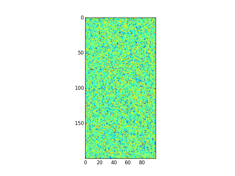
- Create a 2d array of random (you can pick which distribution) noise, of size 200 x 100.
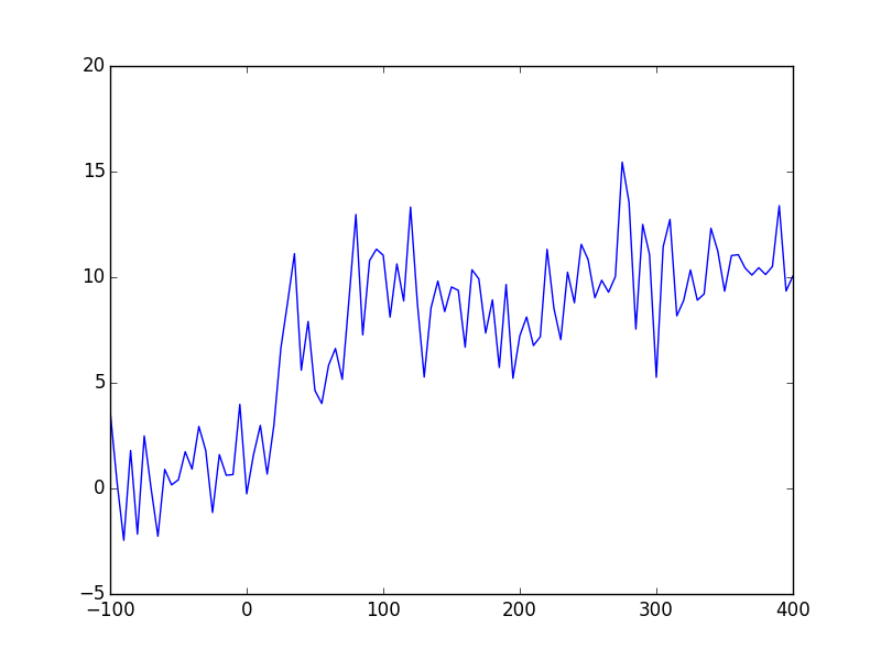
Create the following plots and display them to the screen
- A 1d line plot of the first column of the growth data (~t) vs the signal
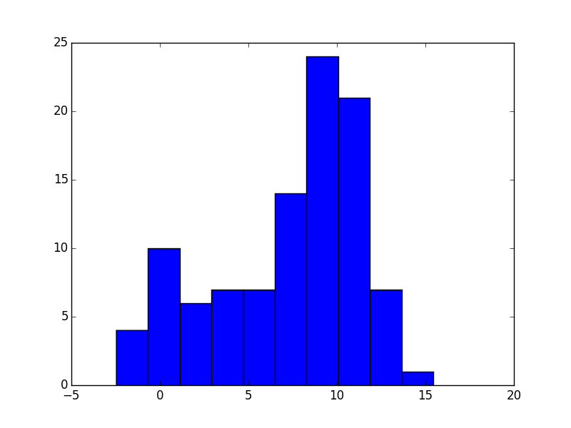
- A histogram of the t >= 0 part of the signal data (i.e. a graphical version
of the binning statistics you printed to the terminal - use
matplotlib’shistfunction. - An image plot (i.e. an image) of the 2d data
Exercise
Loading and generating Numpy arrays is very similar to the exericises in the last section.
All that’s really being added here are some very simple plot functions,
namely plot, hist, and imshow.
For this first example you will either need to call matplotlib’s show
function after each plot is created, or you could create a new figure
for each plot using the figure function, and call show only once
at the end of the script.
Answer
# Practice of basic matplotlib plotting commands

import numpy as np
import matplotlib
matplotlib.use("agg")

import matplotlib.pyplot as plt

import os
ROOT = os.path.realpath(os.path.dirname(__file__))

# Load and generate arrays
arr1 = np.loadtxt(os.path.join(ROOT, "growth_data.csv"), delimiter=",")
arr2 = 3.14 * np.random.randn(200,100) + 66

# Do plotting
# NOTE: Instead of the `savefig` lines, your code should be calling `plt.show()`!
plt.plot(arr1[:,0], arr1[:,1])
plt.savefig("answer_mpl_simple1.png"); plt.clf()

plt.hist(arr1[:,1], bins=10)
plt.savefig("answer_mpl_simple2.png"); plt.clf()

plt.imshow(arr2)
plt.savefig("answer_mpl_simple3.png"); plt.clf()
This should produce the following plots:
Customizing the figure
Most plotting functions allow you to specify additional keyword arguments, which determine the plot characteristics.
For example, a the line plot example may be customized to have a red dashed line and square marker symbols by updating our first code snippet to
plt.plot(arr1d, '--', color="r", marker="s")
(or the shorthand plt.plot(arr1d, "--r"))
Axis labels, legends, etc
Additional figure and axes properties can also be modified. To do so, we need to access figure/axis respectively.
To create a new (empty) figure and corresponding figure object,
use the figure function:
fig1 = plt.figure()
# Now we can modify the figure properties, e.g.
# we can set the figure's width (in inches - intended for printing!)
fig1.set_figwidth(10)
# Then setting the figure's dpi (dots-per-inch) will determine the
# number of pixels this corresponds to...
fig1.set_dpi(300)       # I.e. the figure width will be 3000 px!
If instead we wish to modify an already created figure object,
we can either get a figure object by passing it’s number propery
to the figure function e.g.
f = plt.figure(10) # Get figure number 10
or more commonly, we get the active figure (usually the last created figure) using
f = plt.gcf()
Axes are handled in a similar way;
ax = plt.axes()
creates a default axes in the current figure (creates a figure if none are present), while
ax = plt.gca()
gets the current (last created) axes object.
Axes objects give you access to changing background colours, axis colours, and many other axes properties.
Some of the most common ones can be modified for the current axes without
needing to access the axes object as matplotlib.pyplot has convenience
functions for this e.g.
plt.title("Aaaaarghh")          # Sets current axes title to "Aaaaarghh"

plt.xlabel("Time (s)")          # Sets current axes xlabel to "Time (s)"
plt.ylabel("Amplitude (arb.)")  # Sets current axes ylabel to "Amplitude (arb.)"

# Set the current axes x-tick locations and labels
plt.yticks( numpy.arange(5), ('Tom', 'Dick', 'Harry', 'Sally', 'Sue') )
A note on style
Matplotlib’s default plotting styles are often not considered to be desirable, with critics citing styles such as the R package ggplot’s default style as much more “professional looking”.
Fortunately, this criticism has not fallen on deaf ears, and while it has always been possible to create your own customized style, Matplotlib now includes additional styles by default as “style sheets”.
In particular, styles such as ggplot are very popular and essentially emulate ggplot’s style (axes colourings, fonts, etc).
The style may be changed before starting to plot using e.g.
plt.style.use('ggplot')
A list of available styles may be accessed using
plt.style.available
(on the current machine this holds : ['dark_background',
'fivethirtyeight', 'bmh', 'grayscale', 'ggplot'])
You may define your own style file, and after placing it in a specific folder ( “~/.config/matplotlib/mpl_configdir/stylelib” ) you may access your style in the same way.
Styles may also be composed together using
plt.style.use(['ggplot', 'presentation'])
where the rules in the right-most style will take precedent.
Exercise : trying a new style
Repeat the simple plotting exercise with the "ggplot" style;
to do this, copy and paste the code from the simple plotting exercise
but add the code to change the style to the ggplot style
before the rest of the code.
Answer
To change the style to ggplot, simply add
plt.style.use('ggplot')
after having imported matplotlib.pyplot (as plt).
3d plotting
While matplotlib includes basic 3d plotting functionality (via mplot3d),
we recommend using a different library if you need to generate
“fancy” looking 3d plots.
A good alternative for such plots isa package called mayavi.
However this is not included with WinPython and the simplest route to installing it involves installing the Enthough Tool Suite (http://code.enthought.com/projects/).
For the meantime though, if you want to plot 3d data, stick with the mplot3d
submodule.
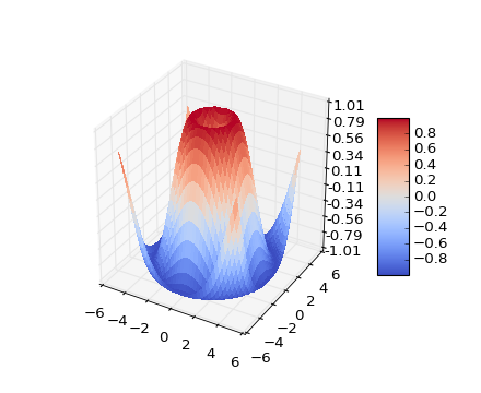
For example, to generate a 3d surface plot of the 2d data (i.e. the “pixel” value would correspond to the height in z), we could use
import matplotlib.pyplot as plt
from mpl_toolkits.mplot3d import Axes3D
fig = plt.figure()
ax = fig.add_subplot(111, projection='3d')
ax.plot_surface(X, Y, Z)
where X, Y, Z are 2d data values.
X and Y are 2d representations of the axis values which can be
generated using utility functions, e.g. pulling an example from the
Matplotlib website,
from mpl_toolkits.mplot3d import Axes3D
from matplotlib import cm
from matplotlib.ticker import LinearLocator, FormatStrFormatter
import matplotlib.pyplot as plt
import numpy as np

fig = plt.figure()
ax = fig.gca(projection='3d')
X = np.arange(-5, 5, 0.25)
Y = np.arange(-5, 5, 0.25)
X, Y = np.meshgrid(X, Y)
R = np.sqrt(X**2 + Y**2)
Z = np.sin(R)
surf = ax.plot_surface(X, Y, Z, rstride=1, cstride=1, cmap=cm.coolwarm,
                       linewidth=0, antialiased=False)
ax.set_zlim(-1.01, 1.01)

ax.zaxis.set_major_locator(LinearLocator(10))
ax.zaxis.set_major_formatter(FormatStrFormatter('%.02f'))

fig.colorbar(surf, shrink=0.5, aspect=5)

plt.show()
Saving plots
Now that we have an idea of the types of plots that can be generated using Matplotlib, let’s think about saving those plots.
If you call the show command, the resulting figure window includes
a basic toolbar for zooming, panning, and saving the plot.
However, as a Pythonista, you will want to automate saving the plot (and probably forego viewing the figures until the script has batch processed your 1,000 data files!).
The command to save the currently active figure is
plt.savefig('filename.png')
Alternatively, if you store the result of the
plt.figure() function in a variable as mentioned above
you can subsequently use the savefig member-function
of that figure object to specifically save that figure, even if
it is no longer the active figure; e.g.
fig1 = plt.figure()

#
# Other code that generates more figures
#
# ...
#


fig1.savefig('figure1.pdf')
Note on formats: Raster vs Vector
The filename extension that you specify in the savefig function
determines the output type; matplotlib supports
- png - good for images!
- jpg (not recommended except for drafts!)
- pdf - good for (vector) line plots
- svg
as well as several others.
The first two formats are known as raster formats, which means that the entire figure is saved as a bunch of pixels.
This means that if you open the resulting file with an image viewer, and zoom in, eventually the plot will look pixelated/blocky.
The second two formats are vector formats, which means that a line plot is saved as a collection of x,y points specifying the line start and end points, text is saved as a location and text data and so on.
If you open a vector format file with e.g. a PDF file viewer, and zoom in, the lines and text will always have smooth edges and never look blocky.
As a general guideline, you should choose to mainly use vector file (pdf, eps, or svg) output for plots as they will preserve the full data, while raster formats will convert the plot data into pixels.
In addition, if you have vector image editing software like Inkscape or Adobe Illustrator, you will be able to open the vector image and much more easily change line colours, fonts etc.
Other annotations
We already saw how to add a title and x and y labels; below are some more examples of annotations that can be added.
You could probably guess most of what the functions do (or have guessed what the function would be called!):
plt.title("I'm a title") # Note single quote inside double quoted string is ok!
plt.xlabel("Time (${\mu}s$)")       # We can include LaTex for symbols etc...
plt.ylabel("Intensity (arb. units)")

plt.legend("Series 1", "Series 2")

plt.colorbar()      # Show a colour-bar (usually for image data).

# Add in an arrow
plt.arrow(0, 0, 0.5, 0.5, head_width=0.05, head_length=0.1, fc='k', ec='k')
The last command illustrates how as with most
most plotting commands, arrow accepts a
large number of additional keyword arguments (aka kwargs) to
customize colours (edge and face), widths, and many more properties.
Exercise : comparing raster and vector formats
Create a new script file (exercise_mpl_raster_vs_vector.py) and create
a simple line plot of y=x^2 between x=-10 and x=10.
Add in labels for the x and y axis; call the x axis, "x (unitless)" and the
y axis “y = x^2” (see if you can figure out how to render the squared symbol, i.e.
a super-script 2; those of you familiar with LaTex should find this easy!).
Save the plot as both a png and pdf file, and open both side-by-side. Zoom in to compare the two formats.
Answer
To generate the x and y data use Numpy’s linspace function for x, and the generate the y data from
the x data.
To render mathematical symbols, use the latex expression: “$x^2$” - if you’re not familiar with LaTex and don’t care about being able to render mathematical expressions and symbols, don’t worry about this!
Otherwise, you might want to read up about mathematical expressions in LaTex.
Use the plt.savefig function to save the figure twice, once with file extension (the end of the
filename) png, and once with extension pdf.
Sub-plots
There are two common approaches to creating sub-plots.
The first is to create individual figures with well thought out sizes (especially font sizes!), and then combine then using an external application.
Matplotlib can also simplify this step for us, by providing subplot functionality. We could, when creating axes, reposition them ourselves in the figure. But this would be tedious, so Matplotlib offers convenience functions to automatically lay out axes for us.
The older of these is the subplot command, which lays axes out in a regular
grid.
For example
plt.subplot(221)        # Create an axes object with position and size for 2x2 grid
plt.plot([1,2,3])
plt.title("Axes 1")

plt.subplot(222)
plt.plot([1,2,3])
plt.title("Axes 2")

plt.subplot(223)
plt.plot([1,2,3])
plt.title("Axes 3")

plt.subplot(224)
plt.plot([1,2,3])
plt.title("Axes 4")
Note that the subplot command uses 1-indexing of axes (not 0-indexing!).
The above could be simplified (at least in some scenarios) using a for-loop,
e.g.
# datasets contains 4 items, each corresponding to a 1d dataset...
for i, data in enumerate(datasets):
    plt.subplot(2,2,i+1)
    plt.plot(data)
    plt.title("Data %d"%(i+1))
Recently, Matplotlib added a new way of generating subplots, which makes it easier to generate non-uniform grids.
This is the subplot2grid function, which is used as follows,
ax1 = plt.subplot2grid((3,3), (0,0), colspan=3)
ax2 = plt.subplot2grid((3,3), (1,0), colspan=2)
ax3 = plt.subplot2grid((3,3), (1, 2), rowspan=2)
ax4 = plt.subplot2grid((3,3), (2, 0))
ax5 = plt.subplot2grid((3,3), (2, 1))
would generate
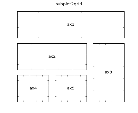 (without the labels!)
Exercise : Adding subplots and insets
Download the image from here: Image File.
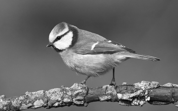
Create a new script (“exercise_mpl_gridplots.py”), and
- Load the image using
matplotlib.pyplot’simreadconvenience function - The image may be loaded into a 3d array - RGB(A) - if so, convert it to grayscale my taking the mean of the first 3 colour channels
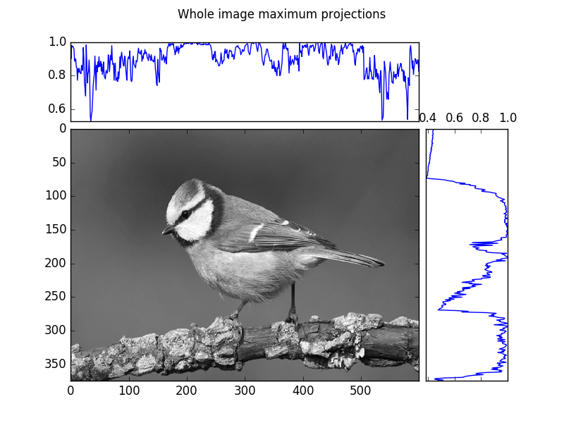
- Create a grid of 3 plots, with the following shape
2x6
---------
| c 8x2 |
------------
|       || |
|   b   ||a|
|  8x6  || |
|       || |
------------
Here,
- a is a maximum projection onto the y axis (2x8 panel)
- b is the full grayscale image (8x6 panel)
- c is a maximum projection onto the x axis (8x2 panel)
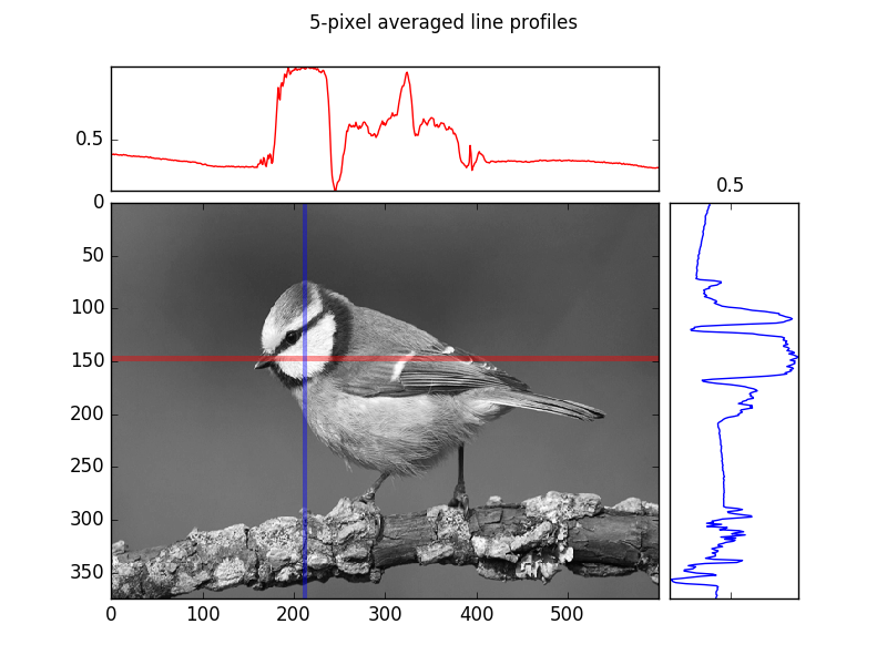
Next create a similar subplot figure but this time, instead of performing maximum projections along the x and y axes, generate the following mean line-profiles:
- A profile along a horizontal line at y=147 averaged over a of width 5 pixels (i.e. averaging from y=145 to 149 inclusive)
- A profile along a vertical line at x=212 averaged over a width of 5 pixels (i.e.
Exercise
The main thing we’re practicing here is the use of the subplottling functionalities in Matplotlib.
Using subplot2grid will make this much easier than trying to
manually position axes in the figure.
Maximum projections and line profile
A maximum projection means for the given dimension (e.g. row or column), extract the maximum value of the image (array) each for row or column.
A basic line profile means given a line (in our case horizontal and vertical lines, which correspond to rows and columns of the array respectively), simply pull out those values and plot them as a 1d plot.
An often more robust version of the simple line profile, is a line profile of finite (> 1 pixel) width that is averaged at each point along the line across the pixels along the width. Put another way, visualize first of all a rectangle instead of a line, and perform a mean-projection of the rectangular (2d) array of values. The resulting 1d array of values is the width-meaned line profile.
If you’d like more information about generating the maximum projections or the line profiles, ask a demonstrator.
Answer
# Create a subplot figure

# NOTE: You shouldn't need the following 2 lines, yet, but they're useful for
# "headless" plotting (i.e. on machines with no display)
import matplotlib
matplotlib.use('agg')

import matplotlib.pyplot as plt
import numpy as np

# "Usual" script folder extraction method (as used in many previous exercises!)
import os
SCRIPT_DIR = os.path.realpath(os.path.dirname(__file__))

# Load the data
im = plt.imread(os.path.join(SCRIPT_DIR, "grayscale.png"))

# Take the mean of the RGB channels (dims are Width, Height, Colour Channels)
# (up to 3 as "Alpha" aka opacity channel also included at index 3)
im = im[...,:3].mean(axis=-1)


# Maximum projections using the Numpy Array max member-function with
# axis keyword argument to select the dimension to "project" along.
maxx = im.max(axis=0)
maxy = im.max(axis=1)#[-1::-1]

def plot_im_and_profiles(im, palongx, palongy, cx = "b", cy = "b"):
    """
    Use a function to do the plotting as we do essentially the same thing
    more than once, ie generate an image plot with the line-profile plots
    above and to the right of the image plot
    """
    # Create 3 axes with specified grid dimensions
    ax_a = plt.subplot2grid((8,10), (2,8), colspan=2, rowspan=6)
    ax_a.plot(palongy, np.arange(len(palongy)), color=cy)
    ax_a.locator_params(tight=True, nbins=4)
    ax_a.xaxis.set_tick_params(labeltop="on", labelbottom='off')
    ax_a.yaxis.set_visible(False)
    ax_b = plt.subplot2grid((8,10), (2,0), colspan=8, rowspan=6)
    ax_b.imshow(im, cmap='gray')
    plt.axis('tight')# ax_b.
    ax_c = plt.subplot2grid((8,10), (0,0), colspan=8, rowspan=2)
    ax_c.plot(palongx, color=cx)
    ax_c.locator_params(tight=True, nbins=4)
    ax_c.xaxis.set_visible(False)
    # Return the axes objects so we can easily add things to them
    # in our case we want to add an indication of where the line
    # profiles are taken from
    return ax_a, ax_b, ax_c

plot_im_and_profiles(im,maxx, maxy[-1::-1])
# Suptitle gives a whole figure a title
# (as opposed to individual axes
plt.suptitle("Whole image maximum projections")
plt.savefig(os.path.join(SCRIPT_DIR, "answer_mpl_subplot1.png"))
# Now add in a "line-profile", width 5 and averaged
# at y ~ 145 and x ~ 210
profx = im[145:150, :].mean(axis=0)
profy = im[:, 210:215].mean(axis=1)[-1::-1]
ax_a, ax_b, ax_c  = plot_im_and_profiles(im,profx, profy, cx="r", cy="b")
# Show the line profile regions using `axvspan` and `axhspan`
ax_b.axhspan(145,150, fc = "r", ec="none", alpha=0.4)
ax_b.axvspan(210,215, fc = "b", ec="none", alpha=0.4)
plt.suptitle("5-pixel averaged line profiles")
plt.savefig(os.path.join(SCRIPT_DIR, "answer_mpl_subplot2.png"))
This generates the following two figures:
Additional exercise resources
If you would like to further practice Matplotlib, please visit this resource.
Scipy : Additional scientific computing modules
Numpy is one of the core modules of the Scipy “ecosystem”;
however, additional numerical
routines are packages in the separate scipy module.
The sub-modules contained in scipy include:
scipy.cluster: Clustering and cluster analysisscipy.fftpack: Fast fourier transform functionsscipy.integrate: Integration and ODE (Ordinary Differential Equations)scipy.interpolate: Numerical interpolation including splines and radial basis function interpolationscipy.io: Input/Output functions for e.g. Matlab (.mat) files, wav (sound) files, and netcdf.scipy.linalg: Linear algebra functions like eigenvalue analysis, decompositoins, and matrix equation solversscipy.ndimage: Image processing functions (works on high dimensional images - hence nd!)scipy.optimize: Optimization (minimize, maximize a function wrt variables), curve fitting, and root findingscipy.signal: Signal processing (1d) including convolution, filtering and filter design, and spectral analysisscipy.sparse: Sparse matrix support (2d)scipy.spatial: Spatial analysis related functionsscipy.statistical: Statistical analysis including continuous and discreet distributions and a slew of statistical functions
While we don’t have time to cover all of these submodules in detail, we will give a introduction to their general usage with a couple of exercise and then a sample project using a few of them to perform some 1d signal processing.
Exercise : Curve fitting
Curve fitting represents a relatively common research task, and fortunatley Python includes some great curve fitting functionalities.
Some of the more advanced ones are present in additional Scikit libraries,
but Scipy includes some of the most common algorithms in the optimize
submodule, as well as the odr submodule, which covers the more elaborate
“orthogonal distance regression” (as opposed to ordinary least squares
used in curve_fit and leastsq).
Load the data contained in the following file
and use the scipy.optimize.curve_fit or scipy.optimize.leastsq (least-squares)
fitting function (curve_fit calls leastsq but doesn’t give as much output!)
to generate a line of best fit for the data.
You shold evaluate several possible functions for the fit including
- A straight line
f(x,a,b) = a*x + b - A quadratic fit
f(x,a,b,c) = a*x^2 + b*x + c - An exponential fit
f(x,a,b,c) = a*e^(b*x) + c
Generate an estimate of the goodness of fit to discriminate between these possible models.
Bonus section
Try the same again with the following data (you should be able to just change the filename!)
You should find that the goodness of fit has become worse. In fact the algorithm used
by Scipy’s optimize submodule is not always able to determine which of the models fits best.
Try using the scipy.odr submodule instead; a guide for how to do this can be found
here
Exercise
General tips:
- Use a function for the fitting; this will allow you to call the same fitting proceedures on multiple files easily!
- Create a dictionary of fitting functions, with their name as the key and the function
as values (see the additional advanced Python section to learn about the
lambdas used here, or stick with defining the functions the usual way, withdef). - Loop over the fitting functions to perform the same operations with each one.
Answer
import numpy as np
import scipy.optimize as scopt
def perform_fitting(filename):
    funcs = {
        'linear'        : lambda x,a,b,c : a*x + b,
        'quadratic'     : lambda x,a,b,c : a*x*x + b*x + c,
        'exponential'   : lambda x,a,b,c : a*np.exp(b*x) + c,
    }

    data = np.fromfile(filename)
    Npoints = len(data)

    taxis = np.arange(Npoints)
    for fname in funcs:

        popt, pcov = scopt.curve_fit( funcs[fname], taxis, data)
        yexact = funcs[fname](taxis, *popt)
        residuals = data - yexact
        ss_err = (residuals**2).sum()
        ss_tot = ((data-data.mean())**2).sum()
        rsquared = 1-(ss_err/ss_tot)

        print("\n\n\nFitting: %s"%fname)
        print("\nCurve fit")
        print("popt:", popt)
        print("pcov:", pcov)
        print("rsquared:", rsquared)

if __name__ == "__main__":
    perform_fitting("curve_fitting_data_simple.txt")
Output
The first part of the quesrtion generates the output below (the last line represents the R^2 goodness of fit statistic for each fit)
Fitting: quadratic

Curve fit
popt: [  0.27742012   0.43227489  24.42625192]
pcov: [[  1.24062405e-04  -2.35718583e-03   7.07155749e-03]
 [ -2.35718583e-03   4.80617819e-02  -1.65474460e-01]
 [  7.07155749e-03  -1.65474460e-01   8.07571966e-01]]
rsquared: 0.99839145357

Fitting: linear

Curve fit
popt: [ 5.70325725  8.61330482  1.        ]
pcov: inf
rsquared: 0.939693857665

Fitting: exponential

Curve fit
popt: [ 19.98312703   0.10003282   2.07108578]
pcov: [[  2.35952209e-03  -5.30270860e-06  -3.10538435e-03]
 [ -5.30270860e-06   1.20524441e-08   6.87521073e-06]
 [ -3.10538435e-03   6.87521073e-06   4.24287754e-03]]
rsquared: 0.999998872202
We see from this that for non-noisy data using curve_fit performs relatively
well (i.e. the data was indeed exponential!).
Bonus section
If we run the same function on the file “curve_fitting_data_noisy.txt”, we get
Fitting: quadratic

Curve fit
popt: [  0.36402064   1.39338512  33.74952291]
pcov: [[  1.16491630e-02  -2.21334100e-01   6.64002296e-01]
 [ -2.21334100e-01   4.51288594e+00  -1.55376545e+01]
 [  6.64002296e-01  -1.55376545e+01   7.58290698e+01]]
rsquared: 0.932781903212

Fitting: linear

Curve fit
popt: [  8.30977729  13.0003464    1.        ]
pcov: inf
rsquared: 0.887804486031

Fitting: exponential

Curve fit
popt: [ 37.66928574   0.08831645  -6.97576507]
pcov: [[  5.63753689e+02  -6.41775284e-01  -6.99939382e+02]
 [ -6.41775284e-01   7.38443618e-04   7.87263594e-01]
 [ -6.99939382e+02   7.87263594e-01   8.90820497e+02]]
rsquared: 0.933020625779
i.e. as far as curve_fit is concerned, both quadratic and exponential are relatively good fits,
and the one that “wins out” will vary depending on the noise present.
However, if we add in the additional odrpack version of the stats
by adding
import scipy.odr as scodr
by the import statements, and the following to the loop over functions:
...
        print("\nODRPACK VERSION")
        funcnow = lambda params, x: funcs[fname](x, *params)
        mod = scodr.Model(funcnow)
        dat = scodr.Data(taxis,data)
        odr = scodr.ODR(dat, mod, beta0 = [1.0, 1.0, 0.0])
        out = odr.run()
        out.pprint()
we also produce
Fitting: quadratic

...

ODRPACK VERSION
Beta: [  0.55201606  -0.63943926  31.30145991]
Beta Std Error: [ 0.08980006  1.10407977  1.93744129]
Beta Covariance: [[ 0.00241881 -0.0263813   0.01923865]
 [-0.0263813   0.36563691 -0.35584366]
 [ 0.01923865 -0.35584366  1.12591663]]
Residual Variance: 3.333886943328627
Inverse Condition #: 0.0020568238964839263
Reason(s) for Halting:
  Iteration limit reached

Fitting: linear

...

ODRPACK VERSION
Beta: [ 9.34657515  3.1507637   0.        ]
Beta Std Error: [ 0.78204438  8.56164287  0.        ]
Beta Covariance: [[  0.14923625  -1.41774486   0.        ]
 [ -1.41774486  17.8865157    0.        ]
 [  0.           0.           0.        ]]
Residual Variance: 4.098155829657788
Inverse Condition #: 0.0437541938307872
Reason(s) for Halting:
  Problem is not full rank at solution
  Sum of squares convergence

Fitting: exponential

...

ODRPACK VERSION
Beta: [ 43.9540789    0.08427052 -17.18528396]
Beta Std Error: [  2.68421883e+01   2.80794795e-02   3.04612945e+01]
Beta Covariance: [[  2.69641542e+02  -2.79919119e-01  -3.04410441e+02]
 [ -2.79919119e-01   2.95072729e-04   3.13666736e-01]
 [ -3.04410441e+02   3.13666736e-01   3.47254336e+02]]
Residual Variance: 2.672077403678681
Inverse Condition #: 8.544672221858744e-06
Reason(s) for Halting:
  Sum of squares convergence
i.e. we see that the residual variance and inverse condition are significantly lower for the exponential fitting (and these values are also more robust to noise).
Exercise : Interpolating data
Another common use of Scipy is signal interpolation.
Background : Interpolation
Interpolation is often used to resample data, generating data points at a finer spacing than the original data.
A simple example of interpolation is image resizing; when a small image is resized to a larger size, the “in-between” pixel values are generated by interpolating their values based on the nearest original pixel values.
Typical interpolation schemes include nearest, linear, and spline interpolation of various degrees. These terms denote the functional form of the interpolating function.
- nearest neighbor interpolation assigns each interpolated value the value of the nearest original value
- linear interpolation assigns each interpolated value the linearly weighted combination of the neighbouring values; e.g. if the value to be interpolated is 9 times closer to original point B than original point A, then the final interpolated value would be 0.1A + 0.9B.
- Spline interpolation approximates the region between the original data points as quadratic or cubic splines (depending on which spline interpolation order) was selected.
Download the data from here:
and use “linear” interpolation to interpolate the data to increase so that the new “x axis” has five times as many points between then original limits (i.e. you’ll resample the data to 5 times the density).
Bonus
Run the interpolation with “quadratic” and “cubic” interpolation also (it helps if your interpolation code was in a function!), and you should see much better results!
Exercise
Use the Numpy load function to load the data (as it was created with save!).
If you plot the data ( data[0] vs data[1] ), you should see a jagged sine curve.
Use the linspace function to create your new, denser x axis data.
After interpolation, you should end up with a slightly smoother sine curve.
Answer
import scipy.interpolate as scint
import numpy as np
import matplotlib.pyplot as plt     # For plotting


def interp_data(data, kind="quadratic"):
    plt.plot(data[0], data[1])

    func = scint.interp1d(data[0], data[1], kind=kind)

    xnew = np.linspace(data[0][0], data[0][-1], num=5*len(data[0]))
    ynew = func(xnew)

    plt.plot(xnew, ynew, '-r')
    plt.title("Using %s interpolation"%kind)
    plt.show()


if __name__ == '__main__':

    data= np.load("data_interpolation.npy")
    for kind in ["linear", "quadratic", "cubic"]:
        interp_data(data, kind=kind)
will produce 3 plots to the screen; the cubic and quadratic version of the interpolation should look much smoother (closer to a real sine curve).
Guided exercise: Signal analysis
As you may not have a background in signal processing, as our last exercise, we’ll you through the process instead of leaving you to generate the code from scratch.
Download the wav file (uncompressed audio) from here Wav File.
This sound file will be the basis of our experimentation with some of the additional Scipy modules
Loading data : scipy.io
scipy.io contains file reading functionality to load Matlab .mat files,
NetCDF, and wav audio files, amongst others.
We will use the wavfile submodule to load our audio file;
import scipy.io.wavfile as scwav
data, rate = scwav.read("audio_sample.wav")
Next we can inspect the the loaded data using a plot (plotting just the first 500 values),
import matplotlib.pyplot as plt
# Create a "time" axis array; at present there are
# `rate` data-points per second, as rate corresponds to the
# data sample rate.
Nsamples = len(data)
time_axis = np.arange(Nsamples)/rate
plt.plot( time_axis[:500], data[:500])
plt.show()
We should see an audio trace that looks something like
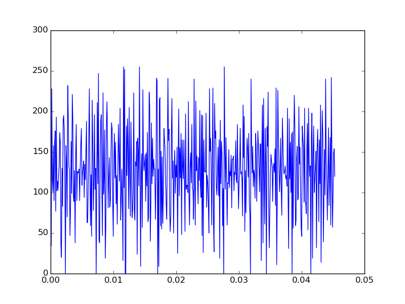
If you have headphones with you and play the audio, you’ll hear a noisy, but still recongnizable sound-bite.
Let’s see if we can improve the sound quality by performing some basic signal processing!
Cleaning the data using : scipy.signal
There are a host of available 1d filters available in Scipy.
We’re going to construct a simple low-pass filter using the
firwin function;
import scipy.signal as scsig

# Calculate the Nqyist rate
nyq_rate = rate / 2.
# Set a low cutoff frequency of the filter: 1KHz
cutoff_hz = 1000.0
# Length of the filter (number of coefficients, i.e. the filter order + 1)
numtaps = 29
# Use firwin to create a lowpass FIR filter
fir_coeff = scsig.firwin(numtaps, cutoff_hz/nyq_rate)

# Use lfilter to filter the signal with the FIR filter
filtered = scsig.lfilter(fir_coeff, 1.0, data)

# Write the filtered version into an audio file so we can see
# if we can hear a difference!
scwav.write("filtered.wav", rate, filtered)
While “manual” verification by listening to the filtered signal can be useful, we would probably want to also analyze both the original signal and the effect the filtering has had.
Spectral analysis : scipy.fftpack and scipy.signal
To analyze a 1d filter, we often generate a periodogram, which essentially gives us information about the frequency content of the signal. The perriodogram itself is a power-spectrum representation of the Fourier transform of the signal; however, this is not a detailed course in 1d signal processing, so if you have no idea what that means then don’t worry about it!
For sound signals, the periodogram relates directly to the pitches of the sounds in the signal.
Let’s generate and plot a periodogram using scipy:
plt.figure()
f, Pxx = scsig.periodogram(data.astype(float), rate)
plt.semilogy(f, Pxx)
plt.xlabel('frequency [Hz]')
plt.ylabel('PSD [V**2/Hz]')
plt.show()
plt.figure()
f, Pxx = scsig.periodogram(filtered.astype(float), rate)
plt.semilogy(f, Pxx)
plt.xlabel('frequency [Hz]')
plt.ylabel('PSD [V**2/Hz]')
plt.show()
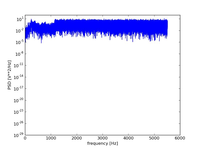
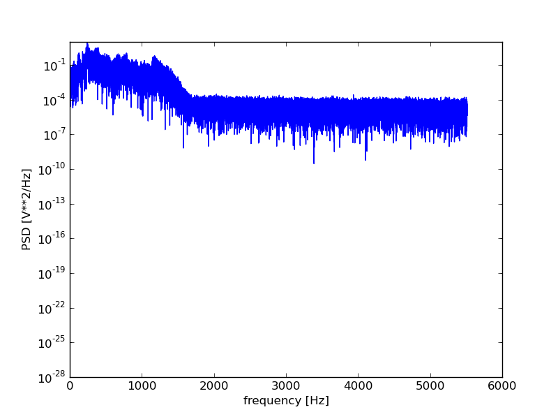
For those wanting more control over the spectral analysis, the fftpack
submodule offers access to a range of Fast-Fourier transform related
functions.
Performing the spectral analysis shows us that the signal did indeed contain a high frequency noise component that the filtering should, at least to some degree have helped remove.
Additional exercise resources
If you would like to further practice Scipy and it’s submodules, please visit this resource.
Optional Sections
Having completed the sections the core Scipy Stack modules, namely Numpy, Scipy, and Matplotlib, you will now be fully equipped to perform data analysis using Python.
However, there are additional core and non-core Scipy packages that might be of use to some of you, as well as non-Scipy packages, for example related to creating user interfaces.
Some of these additional modules are outlined in the following sections. They are intended as optional sections of this workshop, as they are of narrower focus and you will therefore most likely not find all of them useful.
You are encouraged to pick and choose the sections that you deem to be useful for your work and focus on those.
Data wrangling with Pandas
Pandas (pandas) provides a high-level interface to working with
“labeled” or “relational” data. This is in contrast to Numpy that
deals with raw matrices / arrays, and leaves any tracking of
“labeling” up to the developer.
More specifically, pandas is well suited for:
- Tabular data with heterogeneously-typed columns, as in an SQL table or Excel spreadsheet
- Ordered and unordered (not necessarily fixed-frequency) time series data
- Arbitrary matrix data (homogeneously typed or heterogeneous) with row and column labels
- Any other form of observational / statistical data sets. The data actually need not be labeled at all to be placed into a pandas data structure
Full tutorial resources
This page provides a brief introduction to Pandas.
There are many more exhaustive online tutorials available.
A good collection can be found at
the official tutorial page
You are encouraged to check out the material there once you have briefly acquainted yourself with pandas from the information on this page.
Series and Data-frames
To deal with these datasets, Pandas uses two main objects: Series (1d) and
DataFrame (2d).
R users familiar with the data.frame concept will find that the Pandas DataFrame
provides the same functionality plus more.
Reading data from CSV or Excel files
To create a DataFrame object from data in a CSV (Comma Separated Values) file,
Pandas, provides a simple loading function:
df = pandas.read_csv('data.csv')
Similarly a table of data can be read from an Excel Worksheet using
df = pandas.read_excel('workbook.xlsx')
with optional (keyword) arguments like sheetname, header, skiprows to
handle specifying the sheet to load, where column labels (headers)
should be read from, and how many rows to skip before reading (for tables that
start part-way down a spreadsheet).
Getting and Inspecting data
DataFrames contain utility member functions such as head, tail, and
describe to provide a view of the initial rows, last rows, and a summary
of the data they contain.
Specific rows/columns can be queried using column headers, e.g.
if a DataFrame contains the headers ['A', 'B', 'C', 'D']
then column A can be returned as a 1d Series using
df['A']
Standard Python slice notation may also be used to select rows, e.g.
df[:3]
selects the first 3 rows of the DataFrame.
Exercise : Loading and inspecting data
Load and inspect the sample data from the following file
Exercise
Use the pandas.read_excel function to load the spreadsheet, and then call the head,
tail, and describe functions
Strings
Pandas can handle strings in tables of data, as well as numerical values.
For example if we have information such as
Filename,   Cells,  keywords
file1.tif,    120,  normal, rod-shaped
file2.tif,     98,  lysed
file3.tif,     40,  large, rod-shaped
file4.tif,    101,  spotty, rod-shaped
...
in an Excel spreadsheet, this could be loaded into a DataFrame as
described above, and subsequently we can access the keywords column
and query which files contained “rod-shaped” cells:
keywords = pd['keywords']       # Select keywords column as Series
is_rod_shaped = keywords.str.contains("rod-shaped")
Slicing the first few rows would give:
print(is_rod_shaped[:3])
outputs
Filename
file1.tif,   True
file2.tif,   False
file3.tif,   True
Name: keywords, dtype: bool
Using string methods like contains allows us to easily
incorporate string information from tables of data.
For further examples of the types of string operations available see here (a table of available methods is included at the bottom of the linked page).
Cleaning messy data
When working with data that has been entered by using third-party software, or via manual entry, we often encounter entries that are not readily usable within a numerical workflow.
Examples include numbers that are parsed as strings because of mistakes such as accidentally being entered as 10.0.1 (extra “.” at the end), and “NaN” values that are represented using other notation (e.g. “NA”, “??”).
Luckily Pandas import functions like read_csv include keyword arguments
for specifying what nan values look like (na_values).
For example, if the data includes “NA” and “?”, we would use something like
df = pandas.read_csv("file1.csv", na_values=["NA", "??"])
If we need to deal with erroneous representation of numbers, we can first load the data as strings, and then parse the strings into the correct format;
df = pandas.read_csv("file1.csv", na_values=["NA", "??"],
        dtype={"Column 10":str})
specifies that the series labeled “Column 10” should be handled as strings, and subsequently
num_dots = df['Column 10'].str.count("\.")      # Need backslash because count treats "." as regex wildcard otherwise!
wrong_strings = df['Column 10'][num_dots > 1]
right_strings = wrong_strings.str[-1::-1].str.replace("\.", "", n=1).str[-1::-1]
df['Column 10'][num_dots > 1] = right_strings
The unwieldly looking second-last expression is so long because the string method replace
only acts from left to right, so we needed to sandwich it in the str[-1::-1] bits to reverse the
string and then unreverse it, as we stated above that the first “.” was the correct one!
Timestamps
When working with system timestamps expressed in terns of seconds (e.g. Unix timestamps), e.g.
Filename,   Creation time
data1.xlsx,    1387295797
data2.xlsx,    1387295796
data3.xlsx,    1387295743
data4.xlsx,    1387295743
we can easily convert these into datetime data types using:
df['Creation time'] = pandas.to_datetime( df['Creation time'], unit='s')
to produce
Filename,   Creation time
data1.xlsx,    2013-12-17 15:56:37
data2.xlsx,    2013-12-17 15:56:36
data3.xlsx,    2013-12-17 15:55:43
data4.xlsx,    2013-12-17 15:55:43
We can even now use string-like comparison to compare dates!
df = df[df['Creation time'] > '1970-01-01']
(this example selects all rows as they were all created since 1970!).
Plotting a column
Once loaded as described in the previous section, a dataframe can be plotted
using pandas.DataFrame interface to matplotlib;
df.plot()
plots each series (column) of the DataFrame as a separate line.
Exericse : Plot the loaded data
Plot the data that was loaded in the previous exercise.
Saving to CSV or Excel
Much in the same way as a DataFrame be easily loaded from a CSV or Excel
file, it can be written back just as easily:
df.to_csv('foo.csv')
Note: to_csv is a member-function of the DataFrame object, while
read_csv was a module-level function of the pandas module.
Additional exercise resources
If you would like to further practice Pandas, please visit this resource.
Scikit-Image : Image Processing with Python
You might remember from the list of sub-modules contained in `scipy` that it includes `scipy.ndimage` which is a useful Image Processing module. However, `scipy` tends to focus on only the most basic image processing algorithms. A younger module, Scikit-Image (`skimage`) contains some more recent and more complex image processing functionality. For real-world applications, a combination of both (and/or additional image processing modules) is often best. > ## Image Processing: A general overview > > While a full introduction to computational image processing is beyond the > scope of this workshop, below we include some of the main concepts. > > An image is a regular grid of pixel values; a grayscale image will > correspond to a 2d array of values and a colour (RGB) image can be > represented by a 3d array of values, where the dimension corresponding to > colour is of size 3, one per colour channel (sometimes an opacity value is > also included as a 4th colour channel, usually denoted "A" for Alpha). > > ### Segmentation > > As images are just matrices, most of image processing is concerned > with extracting information from these > matrices. However, scenes captured in images are often complex > meaning that they are composed of background(s), foreground objects, > and often several other features. Consequently taking whole-matrix > quantities (like mean, median) is rarely sufficient. > > Instead, we usually need to **segment** an image into regions > corresponding to foreground, which means > objects that we're interesed in, and background which corresponds > to everything else. > > ### Analysis > > Once an image has been segmented, further processing might be > required (such as splitting touching foreground objects). > The final stage in an image processing workflow is to use the > segmentation results to extract quantities of interest. > > These final segmentations can also form the basis of advanced algorithms > such as tracking algorithms if the images are part of a time-series (~film). Very often, good automated images analysis results can be obtained by chaining relatively simple image processing operations. For example, if we were given microscopy images of blood cells with some Leukemic cells, we might want to be able to pick out the Leukemic cells to quantify firstly how many Leukemic cells are present per slide image, and perhaps also quantify other parameters such as their sizes, or circularity. We can see that by performing just a few "simple" image processing tasks (blurring, automatic threshold detection applied twice), we are able to pick out the Leukemic cells nicely. The challenge in quantitative image processing is always in creating these initial segmentation *masks*. Once the regions have been segmented, the useful data can be harvested and plotted. For example, from the above images, we could for example plot the area (in pixels) vs the eccentricity (a measure of how non-circular an ellipse is)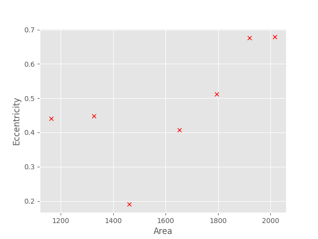 ## Using Scikit-Image
To load get started with Scikit-Image, import the submodule
(the core module is called `skimage`) of interest. For example
to load an image from file, we would use the `io` submodule;
```py
import skimage.io as skio
```
### Loading data with `skimage.io.imread`
```py
im1 = skio.imread("SIMPLE_IMAGE.png")
imstack1 = skio.imread("FILENAME.TIF", plugin="tifffile")
```
Here I first showed a simple image being read from file using the default
`imread` function, followed by a second call using the `plugin` keyword set to
`"tifffile"`, which causes `imread` to use the `tifffile` module. This allows
us to handle multi-page (i.e. multi-stack) tiff files.
`imread` returns a numpy array of either 2 or 3 dimensions, depending on the
file type.
We can then use any normal Numpy operation we wish on the array; e.g.
```py
# Lets output the mean image pixel value
print("The mean of the PNG image is :")
print( im1.mean() )
print("The mean of the TIFF stack (whole stack!) is:")
print( imstack1.mean() )
```
### Displaying data
As we're dealing with Numpy arrays, we can use Matplotlib's imshow function
to display an image (much as we did during the Matplotlib exercises);
```py
import matplotlib.pyplot as plt
plt.imshow(im1)
plt.show()
```
Alternatively, the Scikit-Image team have also added image display functions
directly to `skimage`;
```py
import skimage.viewer as skview
viewer = skview.ImageViewer(im1)
viewer.show()
```
`skimage.viewer` is not as full-featured as `matplotlib`, though new functions
and features are added regularly.
### Getting started with some image-specific processing : basic segmentation
The most basic form of segmentation we can apply is to set a manual
threshold. This is akin to using ImageJ's threshold interface and
manually positioning the threshold position.
```py
the_mask = im1 > 100
```
and that's it! Thresholding is that simple; as `im1` is a Numpy array,
this line will create a **boolean array** stored in the variable `the_mask`,
where each element is `False` if the value of `im1` at the corresponding
location was <= 100, or `True` otherwise.
We can confirm this by viewing our new mask array;
```py
plt.imshow(the_mask)
```
In fact, we can easily overlay the mask on the original image, by using
the `alpha` keyword argument to `imshow`, which sets the transparency of the
image being show;
```py
# Use the `cmap` kwarg to set the colourmap (only works for 2d arrays)
plt.imshow(im1, cmap="gray")
# `the_mask` will be overlaid on `im1` with
# an opacity of 0.4 (maximum 1.0 = fully opaque).
plt.imshow(the_mask, alpha=0.4)
```
We haven't really used any image processing functions; let's remedy that by
automatically determining the threshold value (instead of using a number like
`100` that was plucked from thin air!). One of the most common image thresholding
algorithms, which you may know from ImageJ, is the Otsu automatic threshold
determination algorithm.
To use this in `skimage`, we import the `filters` submodule;
```py
import skimage.filters as skfilt
thresh_val = skfilt.threshold_otsu(im1)
```
at this point, `thresh_val` will hold a single number, which was determined
by the Otsu algorithm to the threshold between what it considered to be
background and foreground pixel intensity values.
We would then generate a mask in the same way as before;
```py
new_mask = im1 > thresh_val
```
and can continue to perform our next round of image processing operations.
### Connected component analysis : `skimage.measure.label`
While having a binary forefound-background mask is a great first step
we are often concerned with multiple objects
In such scenarios, it is usually useful to be able to subsequently determine
per-object quantities, where object is often taken to meaning "connected group
of foreground pixels".
Both `scipy.ndimage` and `skimage.measure` include a connected-component
labelling function called `label`; they work in very similar ways, but
**be careful** that there are subtle differences between.
Basically though, they both work to assign unique labels to each group of
connected foreground pixels (i.e. connected regions of `1`s in the mask array).
```py
object_labels = skmeas.label(new_mask)
```
### Analysis : measuring object sizes and other quantities
Now that we know how to get foreground masks that correspond to individual
objects, let's start extracting some useful quantities.
As performing these kinds of information extractions is such a
common task, `skimage.measure` contains a convenience function
called `regionprops` (which has the same name as the Matlab equivalent
function in Matlab's add-on Image Processing toolbox).
`regionprops` generates a list of `RegionPropery` objects (collections of
properties), which we can then examine. For example
```py
some_props = skmeas.regionprops(object_labels)
# e.g. let's see the area for the first object
print( some_props[0].area )
```
We can also collect specific properties (for plotting, e.g.),
by using a list comprehension (or a for loop);
```py
areas = [p.area for p in some_props]
```
### Exercise : Reproduce the analysis shown at the start of this section
Now that we've covered some of the core image processing techniques,
let's put them into practice by reproducing the results in the
video at the top of the page.
Download the image file:
## Using Scikit-Image
To load get started with Scikit-Image, import the submodule
(the core module is called `skimage`) of interest. For example
to load an image from file, we would use the `io` submodule;
```py
import skimage.io as skio
```
### Loading data with `skimage.io.imread`
```py
im1 = skio.imread("SIMPLE_IMAGE.png")
imstack1 = skio.imread("FILENAME.TIF", plugin="tifffile")
```
Here I first showed a simple image being read from file using the default
`imread` function, followed by a second call using the `plugin` keyword set to
`"tifffile"`, which causes `imread` to use the `tifffile` module. This allows
us to handle multi-page (i.e. multi-stack) tiff files.
`imread` returns a numpy array of either 2 or 3 dimensions, depending on the
file type.
We can then use any normal Numpy operation we wish on the array; e.g.
```py
# Lets output the mean image pixel value
print("The mean of the PNG image is :")
print( im1.mean() )
print("The mean of the TIFF stack (whole stack!) is:")
print( imstack1.mean() )
```
### Displaying data
As we're dealing with Numpy arrays, we can use Matplotlib's imshow function
to display an image (much as we did during the Matplotlib exercises);
```py
import matplotlib.pyplot as plt
plt.imshow(im1)
plt.show()
```
Alternatively, the Scikit-Image team have also added image display functions
directly to `skimage`;
```py
import skimage.viewer as skview
viewer = skview.ImageViewer(im1)
viewer.show()
```
`skimage.viewer` is not as full-featured as `matplotlib`, though new functions
and features are added regularly.
### Getting started with some image-specific processing : basic segmentation
The most basic form of segmentation we can apply is to set a manual
threshold. This is akin to using ImageJ's threshold interface and
manually positioning the threshold position.
```py
the_mask = im1 > 100
```
and that's it! Thresholding is that simple; as `im1` is a Numpy array,
this line will create a **boolean array** stored in the variable `the_mask`,
where each element is `False` if the value of `im1` at the corresponding
location was <= 100, or `True` otherwise.
We can confirm this by viewing our new mask array;
```py
plt.imshow(the_mask)
```
In fact, we can easily overlay the mask on the original image, by using
the `alpha` keyword argument to `imshow`, which sets the transparency of the
image being show;
```py
# Use the `cmap` kwarg to set the colourmap (only works for 2d arrays)
plt.imshow(im1, cmap="gray")
# `the_mask` will be overlaid on `im1` with
# an opacity of 0.4 (maximum 1.0 = fully opaque).
plt.imshow(the_mask, alpha=0.4)
```
We haven't really used any image processing functions; let's remedy that by
automatically determining the threshold value (instead of using a number like
`100` that was plucked from thin air!). One of the most common image thresholding
algorithms, which you may know from ImageJ, is the Otsu automatic threshold
determination algorithm.
To use this in `skimage`, we import the `filters` submodule;
```py
import skimage.filters as skfilt
thresh_val = skfilt.threshold_otsu(im1)
```
at this point, `thresh_val` will hold a single number, which was determined
by the Otsu algorithm to the threshold between what it considered to be
background and foreground pixel intensity values.
We would then generate a mask in the same way as before;
```py
new_mask = im1 > thresh_val
```
and can continue to perform our next round of image processing operations.
### Connected component analysis : `skimage.measure.label`
While having a binary forefound-background mask is a great first step
we are often concerned with multiple objects
In such scenarios, it is usually useful to be able to subsequently determine
per-object quantities, where object is often taken to meaning "connected group
of foreground pixels".
Both `scipy.ndimage` and `skimage.measure` include a connected-component
labelling function called `label`; they work in very similar ways, but
**be careful** that there are subtle differences between.
Basically though, they both work to assign unique labels to each group of
connected foreground pixels (i.e. connected regions of `1`s in the mask array).
```py
object_labels = skmeas.label(new_mask)
```
### Analysis : measuring object sizes and other quantities
Now that we know how to get foreground masks that correspond to individual
objects, let's start extracting some useful quantities.
As performing these kinds of information extractions is such a
common task, `skimage.measure` contains a convenience function
called `regionprops` (which has the same name as the Matlab equivalent
function in Matlab's add-on Image Processing toolbox).
`regionprops` generates a list of `RegionPropery` objects (collections of
properties), which we can then examine. For example
```py
some_props = skmeas.regionprops(object_labels)
# e.g. let's see the area for the first object
print( some_props[0].area )
```
We can also collect specific properties (for plotting, e.g.),
by using a list comprehension (or a for loop);
```py
areas = [p.area for p in some_props]
```
### Exercise : Reproduce the analysis shown at the start of this section
Now that we've covered some of the core image processing techniques,
let's put them into practice by reproducing the results in the
video at the top of the page.
Download the image file:
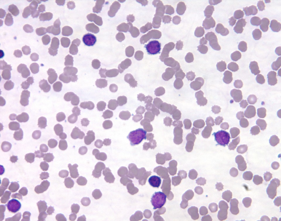 > **NOTE**
>
> This data was saved as JPG which is a compressed image format that uses
> **lossy compression**; but remember -
>
> **KEEP YOUR RAW DATA IN UNCOMPRESSED FORMAT**.
>
> (or lossless compression such as PNG where appropriate).
**Tips**
* Apply a blur filter (i.e. a Gaussian blur).
* In the animation, two rounds of thresholding are applied to the
green channel (index 1!) to produce the masks.
* First a threshold is generated from the whole image
* A second threshold is generated from only the pixels that were
below the first threshold value (white background!)
* Once the final mask is generated, use a `label`ling algorithm...
* `regionprops` contains both `area` and `eccentricity` values for
each region.
#### Manually extracting region properties
If the property we are interested in is not present in the output of
`regionsprops`, we can also calculate the propery ourselves.
There are several relatively straight-forward ways of doing this,
namely to use a utility function like `scipy.ndimage`'s
`labeled_comprehension`
or alternatively a list comprehension or for loop over the label values.
For example we could get the object areas using
```py
areas= [ (object_labels == l).sum()
for l in range(1, object_labels.max()+1) ]
```
or equivalently
```py
areas = []
for l in range(1, object_labels.max() + 1):
current_obj = object_labels == l
areas.append( current_obj.sum() )
```
### Exercise : Counting and measuring "blobs" within blobs
Download the image file:
> **NOTE**
>
> This data was saved as JPG which is a compressed image format that uses
> **lossy compression**; but remember -
>
> **KEEP YOUR RAW DATA IN UNCOMPRESSED FORMAT**.
>
> (or lossless compression such as PNG where appropriate).
**Tips**
* Apply a blur filter (i.e. a Gaussian blur).
* In the animation, two rounds of thresholding are applied to the
green channel (index 1!) to produce the masks.
* First a threshold is generated from the whole image
* A second threshold is generated from only the pixels that were
below the first threshold value (white background!)
* Once the final mask is generated, use a `label`ling algorithm...
* `regionprops` contains both `area` and `eccentricity` values for
each region.
#### Manually extracting region properties
If the property we are interested in is not present in the output of
`regionsprops`, we can also calculate the propery ourselves.
There are several relatively straight-forward ways of doing this,
namely to use a utility function like `scipy.ndimage`'s
`labeled_comprehension`
or alternatively a list comprehension or for loop over the label values.
For example we could get the object areas using
```py
areas= [ (object_labels == l).sum()
for l in range(1, object_labels.max()+1) ]
```
or equivalently
```py
areas = []
for l in range(1, object_labels.max() + 1):
current_obj = object_labels == l
areas.append( current_obj.sum() )
```
### Exercise : Counting and measuring "blobs" within blobs
Download the image file:
 * Use the segmentation method outlined above to count the number of nuclei
(big blue-green blobs) in the image
* Also create a histogram of their size distribution
* Try and see if you can find out how to *exclude nuclei touching the edges*
* Count the number of dark spots inside each cell and plot the distribution of dark spot number.
**Bonus**
* As is usually the case, your segmentation will most likely not 100% match your "mental model" of
how it should look as the data is not perfect!
See if you can find a filter or combination of filters that enhance your final segmentations.
* Use either a limit on minimal size or some other technique to include only dark spots above 3x3 pixels
in size (as smaller dark spots are likely to be noise).
### Additional segmentation: The Watershed transform
Often the actual objects represented in our images touch (or appear to),
causing them to be labelled by the same label during the connected component
analysis.
In these types of scarios, might be able to use an algorithm known as the
Watershed transform
to split touching objects.
Note however, that this won't solve all situations with touching objects, and
in some situations the objects simply won't be resolvable, whilst in others
a different strategy for splitting object might be needed.
To apply the watershed transform, import the `skimage.morphology` submodule,
```py
import skimage.morphology as skmorph
import skimage.feature as skfeature
import scipy.ndimage as ndi
# First generate a distance transformed image
dist = ndi.distance_transform_edt(im1)
# Next generate "markers": regions we are sure belong to different objects
local_maxi = skfeature.peak_local_max(
dist, indices=False, footprint=np.ones((3, 3)),
labels=new_mask)
markers = ndi.label(local_maxi)[0]
# Lastly call the watershed transform - it takes the distance transform
# and the markers as inputs (plus optionally the new_mask to delineate objects
# from background)
new_labels = skmorph.watershed(-dist, markers, mask=new_mask)
```
### Additional exercises?
Image processing techniques are specific to the task being tackled; the previous exercise, while possibly being
of interest to some of you, will by no means be useful to all.
Instead of working on additional contrived exercises, please now try and perform image processing
that is useful to you using your own data (or find similar data online).
* Use the segmentation method outlined above to count the number of nuclei
(big blue-green blobs) in the image
* Also create a histogram of their size distribution
* Try and see if you can find out how to *exclude nuclei touching the edges*
* Count the number of dark spots inside each cell and plot the distribution of dark spot number.
**Bonus**
* As is usually the case, your segmentation will most likely not 100% match your "mental model" of
how it should look as the data is not perfect!
See if you can find a filter or combination of filters that enhance your final segmentations.
* Use either a limit on minimal size or some other technique to include only dark spots above 3x3 pixels
in size (as smaller dark spots are likely to be noise).
### Additional segmentation: The Watershed transform
Often the actual objects represented in our images touch (or appear to),
causing them to be labelled by the same label during the connected component
analysis.
In these types of scarios, might be able to use an algorithm known as the
Watershed transform
to split touching objects.
Note however, that this won't solve all situations with touching objects, and
in some situations the objects simply won't be resolvable, whilst in others
a different strategy for splitting object might be needed.
To apply the watershed transform, import the `skimage.morphology` submodule,
```py
import skimage.morphology as skmorph
import skimage.feature as skfeature
import scipy.ndimage as ndi
# First generate a distance transformed image
dist = ndi.distance_transform_edt(im1)
# Next generate "markers": regions we are sure belong to different objects
local_maxi = skfeature.peak_local_max(
dist, indices=False, footprint=np.ones((3, 3)),
labels=new_mask)
markers = ndi.label(local_maxi)[0]
# Lastly call the watershed transform - it takes the distance transform
# and the markers as inputs (plus optionally the new_mask to delineate objects
# from background)
new_labels = skmorph.watershed(-dist, markers, mask=new_mask)
```
### Additional exercises?
Image processing techniques are specific to the task being tackled; the previous exercise, while possibly being
of interest to some of you, will by no means be useful to all.
Instead of working on additional contrived exercises, please now try and perform image processing
that is useful to you using your own data (or find similar data online).
Creating Graphical User Interfaces (GUIs) with QT in Python
There are several GUI frameworks that one can use when working with Python; one of the most actively developed and widely supported is PyQt (now PyQt5).
What is Qt?
Qt is a cross-platform (Windows, Linux, OS X, Android and others) application framework - it does more than generate UI widgets and dialogs, but that is one of it’s biggest use scenarios.
Qt has been developed by several companies (Trolltech, Nokia, Digia), and as a result is a very mature library with a large user-base.
As mentioned, Qt does much more than creating GUI elements, including Networking, Multimedia, SQL (database), and Webkit (web content rendering), with add-on modules for things like Bluetooth and NFC, Hardware sensors, and GPS positioning service access.
A sample…
- Open the windows file expolrer,
- navigate to the WinPython root directory (~
"C:\WinPython") - Double click the Spyder application to launch it (it might take a while to load)
- Drumroll…
Tadaaaa!!
This is the kind of application that can be written with PyQt. In fact, even the Matplotlib plot windows that you have been using use PyQt (and it is possible to embed these “widgets” in bigger PyQt applications).
There are many other examples - see here for a few : https://wiki.python.org/moin/PyQt/SomeExistingApplications .
We will focus on using Qt for relatively simple GUI creation tasks for now though!
Hello world (with Qt)
We will begin by creating a simple Hello, World program.
The main component of any PyQt5 application is the QApplication object. Usually this is passed
command-line arguments using sys.argv:
import sys
from PyQt5.QtWidgets import QApplication

app = QApplication(sys.argv)
Next we create all windows, dialogues etc, and then call app.exec_()
(often wrapped in sys.exit to capture the return code):
import sys
from PyQt5.QtWidgets import QApplication, QWidget

app = QApplication(sys.argv)

w = QWidget()
w.resize(400, 200)
w.setWindowTitle("Hello, World!")
w.show()

sys.exit( app.exec_() )
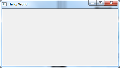
What happened here? PyQt (and the underlying Qt C++ library) work with classes, and GUI elements are connected with an event-driven interface using “signals” and “slots”.
What we did in the code above is to
- create a QApplication object (which is needed for all Qt applications)
- Create a simple QWidget object (the base class for all widgets)
- Change the size and title of the widget
showthe widget- …and lastly, we started the QT event-loop by calling
exec_on our application object.
Pre-made dialogs
However, before we start learning about writing custom file saving dialog, or colour selection widget, be aware that common dialogs like these have already been created for us!
Along with simple message and warning boxes, Qt provides very simple ways to get a file name or file list from the user as well as colour, time, and others like Font selection input, and progress.
Example: QFileDialog
As an example of how easy using one of these dialogs can be, consider the case of wanting to get a file name from the user, for an existing file that will then be opened by the program.
It turns out that this is a simple “one-liner” in PyQt5 (after imports and creating the
QApplication object).
from PyQt5.QtWidgets import QApplication, QFileDialog

app = QApplication([])
# NOTE: This time we don't need to start the event loop!
filename = QWidgets.QFileDialog.getOpenFileName()
or, adding a little more customization,
from PyQt5.QtWidgets import QApplication, QFileDialog

app = QApplication([])
filename = QtWidgets.QFileDialog.getOpenFileName(None, "Select Image file", "", "Images (*.tif)")
Note
While it’s not immediately apparent, this code exposes an additional intricacy related to classes/objects. We didn’t have to create a QFileDialog object, in order to be able to use
getOpenFileNamewhich is a member function of the QFileDialog class. This is becausegetOpenFileNameis a special type of member function, called a static member function. Roughly speaking, unlike a normal member function that has access to object data (remember an object is an instance of a class), static member functions operate at the class level, meaning that they don’t have access to any object-specific data.
Exercise : Getting an output folder location
Try and find out how to create a dialog that show’s a typical “select folder” interface (which we might use for example to get a user to select the output destination for a script).
Once the output folder has been selected, create a simple text file in the folder called
dummy_data.txt, containing the text "Hello! I'm a dummy data file!"
Creating custom dialogs
Our Hello World example contained some of the most basic elements of a QT application; the QApplication object and a simple widget. However, most of the time we want to use common widgets like buttons and text areas. Most of these are predefined in QT, and we will list some below.
Before we do however, let’s quickly learn about how these widgets are going to talk to each other and actually do stuff!
Signals and Slots
In the QT framework, when a button is pressed, or a text field edited, a signal is emitted by the corresponding widget.
To get our application to do something when that signal is emitted, we need to connect the signal to a slot.
Let’s see how this is done in our first example of adding a GUI element.
Adding standard GUI elements
Now that we can display a simple dialog, it’s time to add in some simple GUI elements (aka widgets).
Pushbutton
import sys
from PyQt5.QtWidgets import QApplication, QPushButton

app = QApplication(sys.argv)

w = QPushButton("Press me")
w.resize(400, 200)
w.setWindowTitle("button")
w.show()

def my_first_slot():
    print("I got clicked!")

w.clicked.connect(my_first_slot)

sys.exit( app.exec_() )
As we can see we replaced the QWidget with a QPushButton instance.
Also as mentioned in the section above on signals and slots, we added
a function to act as a slot which we then connected to the
QPushButton’s clicked signal, by calling clicked.connect on the
QPushButton object, and passing the function we want to be the slot
as the first argument.
The QPushButton object’s most commonly used (built-in) signal is clicked for
when the button is clicked; others include pressed for when the button is
pressed down, and released when the button is released.
For more details about signals and slots in general, see here:
http://pyqt.sourceforge.net/Docs/PyQt5/signals_slots.html
The full list of class functions etc for the QPushButton can be found here http://doc.qt.io/qt-5/qpushbutton.html
NOTE
The PyQt5 documentation mainly links to the Qt5 (C++) documentation, as PyQt5 simply “wraps” the C++ library. This means that most of the C++ functions and classes are “roughly the same” as the Python versions.
Edit box
import sys
from PyQt5.QtWidgets import QApplication, QLineEdit

app = QApplication(sys.argv)

w = QLineEdit("I can be edited!")
w.setWindowTitle("line edit")
w.show()

def show_change(text):
    print("CHANGED: ", text)

w.textChanged.connect(show_change)

sys.exit( app.exec_() )
List box & Select box
A list box (QListBox) displays a list of data that can be selected,
while a select box QComboBox shows a button which when clicked
presents a drop-down list.
Slider & Spinners
Sliders (QSlider) and spinners (QSpinBox) are used to set numerical data; both have
minimum and maximum values, though spinners also (optionally) allow arbitrary number input.
Progress bar
A progress bar (QProgressBar) is a visual feedback of the progress of a processes; we’ve doubtlessly
all spent some amount of time watching little bars filling!
QProgressBars can be determinate (ie showing a concrete value) or indeterminate, in which case the indicator slides back
and fore to indicate that the exact progress is unknown.
Layout
So far we have shown single widgets in their own windows. However, most User Interfaces have more complex layouts.
Laying out widgets in Qt can be achieved in one of two main ways
- Using a layout designer; ie a GUI created for designing GUI layout! This generates an intermediate file which is then loaded by PyQt.
- Coding the layout into the source code.
For small to medium complexity layout projects, coding the layout directly is often faster than using the layout designer, and we will focus on this approach here.
While we can position widgets using “absolute positioning” within a dialog, this is not usually recommended as e.g. resizing the dialog will result in a strange looking layout.
Instead, using “layouts” is preferred, as these automate much of the positioning, and reposition widgets if the window is resized.
Horizontal & Vertical
The two most basic layouts are horizontal (QHBoxLayout) and veritcally (QVBoxLayout) aligned widgets.
Note that layouts can be nested, meaning that the first item in a vertical layout can be a horizontal layout etc.
Grid
In order to create a grid of widgets, Qt provides a useful QGridLayout class.
Advanced layouts
Even more advanced layouts are possible through the use of e.g. the QMainWindow class, which provides a main widget area, a menu area, toolbar area etc.
Exercise : build your own!
Instead of telling you to build some dialog with widgets and functionality that has no relevance to you, try and think of a simple(ish) GUI project to get started with PyQt; if you’re struggling for inspiration, start off by copying and slightly editing the examples listed above.
If you’re really stuck, then try the following:
- Create a dialog window and add a slider and a pushbutton
- When the button is pressed, create a matplotlib plot of a sin curve of period specified by the slider.
NOTE: you will need matplotlib.interactive(True) in order to use Matplotlib
with PyQt (it stops Matplotlib trying to start it’s own event loop!).
- As a bonus, add more sliders for amplitude and additional noise component of the plot
- Try creating a tabbed dialog where the settings are in the first tab, and the output in the second.
Additional advanced Python
The following concepts are less frequently needed than those in the first section of this workshop.
However they are nonetheless useful for certain scenarios, and included here for those of you who might find them useful.
Installing modules
You should already be familiar with how to use a module, and all of the modules that you will need for this workshop are included in the WinPython install.
However, for completeness we will briefly mention the simple install
process for new modules; using pip.
pip comes as standard with Python as of 3.4, and allows you to search the
online Python Package Index (PyPI) as well as install packages from PyPI.
From the command line, we can
- Query the (online) Python Package Index, e.g.
pip search memory - Install a package, e.g.
pip install memory_profiler - Remove an installed module, e.g.
pip uninstall memory_profiler
NOTE (Windows):
If the pip executable isn’t recognized by the terminal
the above commands can be replaced by e.g. python -m pip search memory.
Note however, that unless the module is only reliant on Python, the install process may run into dependency problems (e.g. needing a C++ development environment to be set up in order to compile included C++ code).
Command-line arguments & interaction
Command line arguments : sys.argv
Python can read inputs passed to it on the command line by using the
sys module’s argv
attribute (module variable):
print(sys.argv)
If we place that statement in a file (called, e.g. “test_inputs.py”), and run the file with Python as usual:
python test_inputs.py
the output would be the list [ "test_inputs.py" ];
i.e. the first element of argv
(which is a list), is always the name of the script.
Subsequent command-line arguments (separated by spaces) will appear
as additional elements in the list.
For example if we call the script with
python test_inputs.py Hello 2 you
the output (contents of sys.argv) would be
["test_inputs", "Hello", "2", "you"].
This highlights that all command line inputs are interpreted as
strings; if you wish to pass in a number, you would need to convert
the string to a number using either float(STRING) or int(STRING),
where STRING could be "2", "3.14", or sys.argv[2] if the 2nd command
line argument (after the script name) were a number.
Advanced command-line input interfaces
More advanced command-line input interfaces can be created by using
a module such as
argparse
which allows for
- flags (like
-hfor help) - optional arguments
- keyword arguments
- …and many more functionalities!
Interactive input : input
As well as generating terminal output with the print function, we
are also able to read input from the terminal with the
input
function;
for example
some_stuff = input("Please answer yes or no:")
would cause the script (when run), to pause, display the prompt text (i.e.
the first argument to the input function), and then wait for the use to
enter text using the keyboard.
Text entry would finish when the enter key is pressed.
Advanced interactive input
More advanced interactive terminal interfaces are also possible with Python.
The
cmd
module, for example, allows the creation of interactive
commands session, where the developer maps functions he has written to
“interactive commands” which the user can then call interactively (including
features such as interactive help, tab-completion of allowed commands,
and custom prompts.
Decorators : Applying functions to functions
A decorator is a way to “dynamically alter the functionality of a function”. On a practical level, it amounts to passing a function into another function, which returns a “decorated” function.
Why would we want to do such as thing?
Consider the following simple example; we have a number of functions that generate return values;
def add(a, b):
    return a + b

def subtract(a, b):
    return a - b

def multiply(a, b):
    return a * b

def divide(a, b):
    return a / b
Now we want a clean and simple way of turning all of these functions into more “verbose” versions, which also print details to the terminal.
For example when we call add( 10, 2) we want the terminal to read:
Adding 10 and 2 results in 12
Without knowing about decorators, we might think we need to re-write all of our functions. But, as our modification is relatively straight forward to turn into an algorithm, we can instead create a decorator function:
def verbose(func):
    def wrapped_function(a, b):
        # Access the special __name__ attribute to get a function's name
        name   = func.__name__
        result = func(a,b)
        print("%sing %0.2f and %0.2f results in %0.2f"%(name, a, b, result))
        return result
    return wrapped_function
which we the use to decorate our previous function definitions:
@verbose
def add(a, b):
    return a + b

@verbose
def subtract(a, b):
    return a - b

@verbose
def multiply(a, b):
    return a * b

@verbose
def divide(a, b):
    return a / b
E.g. then calling each of these on 10 and 2 as inputs gives:
adding 10.00 and 2.00 results in 12.00
subtracting 10.00 and 2.00 results in 8.00
multiplying 10.00 and 2.00 results in 20.00
divideing 10.00 and 2.00 results in 5.00
Note that the decorator syntax, where we use the @ symbol followed by the decorator function name, and then define the function to be decorated, is the same as
add = verbose(add)
i.e. we are calling the decorator function (here called verbose) on the
input function (add), which returns a wrapped version of add, and we
assign it back into add.
The reason that the decorator syntax (@) was created is that the core Python developers decided that having to first define a function and then apply the decorating syntax would be confusing, especially when dealing with large function definitions or class methods (yes, decorators can also be applied to class methods!).
Lambdas : ~ One-line function definitions
A quick but useful additional python construct is the lambda.
Lambdas a one-line function definitions, which can be extremely
useful to remove the need to create a full function definition for
an almost trivial function.
Let’s look at an example of when this might be useful.
There is an in-built function called filter that is used to filter
lists; the help doc for filter is:
filter(function or None, iterable) --> filter object

Return an iterator yielding those items of iterable for which function(item)
is true. If function is None, return the items that are true.
Given a list of files, we might want to use this function to select only files ending in a specific extension.
However, to do so we need to pass in a function that takes a
filename as an input and returns True or False indicating if the
filename ends in the desired extension. We could now go ahead and define
such a function, but it really is a trivial function and a more efficient
approach is to use a lamba:
# e.g. file list
file_list = ["file1.txt", "file2.py", "file3.tif", "file4.txt"]
text_files = filter( lambda f : f.endswith("txt"), file_list)
Another example of a function that requires another function as an input
is non-standard sorting using sorted, in which case we can pass in a custom “key” function
that is used to extract a sort “key” from each item:
print( sorted(["10 kg", "99 kg", "100 kg"] ))
print( sorted(["10 kg", "99 kg", "100 kg"] , key=lambda k : float(k.split()[0]) ))
outputs
['10 kg', '100 kg', '99 kg']
['10 kg', '99 kg', '100 kg']
Generators and the yield statement
A generator is something that is iterable, and yet the values that are iterated over do not all exist in memory at the same time.
In fact, those of you who attended the Introductory course will have seen a generator without knowing it, when we covered reading data from a file, and you should have just made use of this above above!
There, the last method shown for iterating over a file was (roughly)
for line in open("filename.txt"):
    print(line)
However, what we didn’t mention, was that this approach provides sequential access to the file being read meaning that only one line of the file is loaded into memory per iteration.
This is in contrast to
lines = open("filename.txt").readlines()
for line in lines:
    print(line)
where we read all of the file into memory using readlines.
Under the hood, a file object is a generator, meaning that
for each iteration in for line in <fileobject> the file object
yields the next line of the file.
Similarly, the last comprehension expression we encountered, i.e. the tuple comprehension, yields the value of each list item squared, without loading all of the new values into memory.
Any function where we iterate over something can be converted to a
generator; instead of creating a list/tuple etc in the function
we we use the yield statement instead of return at the end of the
function.
For example consider a simple squared function that takes a list and
generates a new list of squared values:
def squared(list_in):
    list_out = []
    for val in list_in:
        list_out.append(val * val)
    return list_out
To convert this into a generator function we might write
def squared(list_in):
    for val in list_in:
        yield val * val
Running the first version through a memory-profiler,
In [1]: %memit l1 = squared(range(10000000))
peak memory: 391.05 MiB, increment: 367.12 MiB
we see that we create almost 400MB of data in memory by running the traditional function (as we’ve created 10,000,000 numbers - and each is quite a bit larger than the 8 bytes needed for the value alone as Python objects are more than just data!)
By using the generator version of the function instead, we get
In [2]: %memit l2 = squared(range(10000000))
peak memory: 23.80 MiB, increment: 0.10 MiB
i.e. very little additional memory is used!
Can we still use the resulting generator as we would a list? The answer is, most of the time… by which I mean that many functions where we don’t need the list to be all in-memory will work, e.g.
print(sum(l2))
will output 333333283333335000000, but only once, as generators are iterable once and only once.
If we want to call another function on the generator, we would
need to recreate it (i.e. set e.g. l2 = squared(10000000) again).
The bottom line is that generators are useful for specific memory-critical functionalities, such as working with data that is too large to fit in memory.
Exercise : Using generators
Create a script file (“exercise_generators.py”) to evaluate the sum of the squares of the first 1,000,000,000 integers (1 billion or 10E9).
As this is a large number you will at best be barely able to store all of these values in memory at the same time (if each integer were represented using 64 bit / 8 byte this would require at least 8 GB RAM, which is roughly the total amount of RAM a standard current standard desktop PC has!).
NOTE: This will take a couple of minutes to execute!.
While you’re waiting for this to finish running, it’s worth mentioning that
the equivalent functionality in C++ is about 20 times faster; but getting C++
to do this is significantly more difficult (even for such a relatively simple task)
as it involves using the non-standard __int128 compiler extension, which requires
creating a custom output stream operator (to print the result to the screen)!
Nonetheless, for problems involving very simple operations repeated many many times, lower level languages such as C++ may be better suited.
Luckily for us, we don’t need to choose! We can have our cake and eat it…
Beyond Pure Python: When and how
Low-level language purists argue that Python is extremely slow compared with e.g. C, C++, Fortran, or to a lesser extent, Java.
While it is true that Python is slow compared with these languages (typically on the order of 10-40 times slower), pure Python isn’t designed to compete with these languages for speed.
Instead Python prioritizes readability, code design, and simplicity.
That said, there is a large community of Python developers who devote their time to optimizing Python in many ways. These include
- Just-In-Time (JIT) compilers like PyPy, and Pyston (by the Dropbox team)
- Stackless Python which adds “microthreading” for easy thread support
- Multiple ways of interacting with C & C++
ctypes: C “foreign function library” built into Python often used for wrapping c libraries in Pure Python- Cython : writing C/C++ code with Python syntax - cross-compiles “Cython” code to c/c++ which can then be imported into Python
- Others inc.
swig,scipy.weave(Py2), Boost.Python
- Support for GPU programming using e.g. PyOpenCL, CUDA Python
- Specialist libraries like Numba
Using a compiled module
Before you get carried away with these hybrid approaches and/or start to think you might need
to write your whole project using a lower-level language, consider the small snippet below that
demonstrates some simple arithmetic operations in a for-loop:
def simple(amp, N):
    out = []
    for i in range(N):
        val1 = amp * math.sin(i)
        val2 = (abs(val1) - 1)**2
        out.append(val2*val1)
    return out

simple(0.1, 10000)
Ie here we perform some relatively basic mathematical operations
(sin, abs, multiplication, exponentiation, etc),
inside a for loop, looped 10,000 times.
For-loops are one of Python’s common speed bottlenecks compared with low-level languages, so this can be considered to be a relatively representative snippet.
Benchmark results
Running this code using the Numpy module, we get the following statistics:
Numpy:   0.000417 seconds / "loop iteration" (uses matrix operations)

Execution time relative to numpy version (small is good!)

Cython versions
For loop                             :   10.09
List comprehension                   :   15.05
With Basic Cython type declarations  :    5.13
 + return type declarations          :    5.07
 + using cmath abs & sin             :    1.27
 + removed bounds checking           :    1.26

Normal Python
Numpy (vectorized)                   :    0.97
Basic for loop                       :   13.46
List comprehension                   :   17.23

Basic C++
Growing vector                       :    1.44
Pre-assigned vector                  :    1.36

C++ with O2 (optimization) flag
Growing vector                       :    0.97
Pre-assigned vector                  :    0.92

C version with O2                    :    0.89
So the Numpy version (and the best Cython versions!) are faster than the basic Pure C++ version!
This is possible because Numpy is not a pure-python library; all of the basic operations are implemented in c, and wrapped in Python to provide a Python object interface to a load of really fast numerical algorithms!
As this still incurs some overhead, applying optimization flags to the C++ and C version mean these versions are still the fastest.
Using Cython
If someone else (like the Numpy development team!) hasn’t already written the speed-critical functions you need in C/C++ etc for you, there is a gentle way of optimizing your Python code using Cython to perform incremental optimization.
We mentioned Cython above as a way of interfacing with C++. Cython basically converts pure Python into C/C++ and automatically create a Python compatible module from the output.
This means that pure Python is valid Cython code. In fact, by just running Cython on pure python we already obtain a small increase in speed, often of about 10-20%.
By adding in additional Cython-specific information, such as type declarations (and removing calls to Python functions), Cython is able to further optimize your Python code for you.
For example, the optimized Cython version (which operates faster than the unoptimized Pure C++ and almost as fast as the highly optimized Numpy code) is identical to the Python version, featuring just a few Cython specific decorators:
from libc.math cimport sin, abs
@cython.locals(amp=cython.double, N=cython.int, out=list,
    val1 = cython.double, val2 = cython.double)
@cython.returns(list)
def cython_version(amp, N):
    out = []
    for i in range(N):
        val1 = amp * sin(i)
        val2 = (abs(val1) - 1)**2
        out.append(val2*val1)
    return out
That’s it!
The function definition itself is almost identical (except that we switched to the
c math library version of sin and abs), and all we needed was three additional lines;
from libc.math cimport sin, abs
to import the c library functions for sin and abs (so that Cython doesn’t have to switch back to the Python library to call the Python versions of these functions!), and
@cython.locals(amp=cython.double, N=cython.int, out=list,
    val1 = cython.double, val2 = cython.double)
@cython.returns(list)
i.e. two special cython module decorators, locals and returns, that are used to specify the
data types in the local variables and the return variables so that Cython can convert the
Python code to c code. Cython knows how to deal with for loops and Python list conversions.
Not much to add for a more than 10-fold speed increase!
And yet we’ve also been able to still write valid Python code in doing so.
This highlights how we can incrementally add cython annotation to Python code to make it run faster; so if you have a nicely written Python module that has a speed bottleneck that has to be addressed, no need to replace the whole thing with c code - you can simply add in a few cython library lines and run the code through cython to produce an optimized, compiled version of the same code!
Cython also already contains a special cimport numpy directive to allow
operations involving Numpy arrays to be optimized using Cython.
Object-Oriented Programming and Python
To quote one of the first sentences from the wikipedia page on Python:
Python supports multiple programming paradigms, including object-oriented, imperative and functional programming or procedural styles.
In the Introductory notes I also referred to modules functions as well as member functions.
These bits of jargon are related; everything in Python is an object.
In the context of programming, objects
“…are data structures that contain data, in the form of fields, often known as attributes; and code, in the form of procedures, often known as methods.” https://en.wikipedia.org/wiki/Object-oriented_programming
Everything in Python is an object (even functions!)
Every entity in a python script has both data associated with it, and functions.
For example, even the most basic seeming data is an object:
print( (1).__class__ )
yields int - ie the class name attribute of the number 1 is int (the parentheses are needed to distinguish the “.” from a decimal sign!).
Note that this is different from basic programming concept of data type!
As proof, the full list of member functions for our number are:
bit_length   denominator  imag         real
conjugate    from_bytes   numerator    to_bytes
i.e. functions to e.g. get the real and imaginary parts of the number, as well as return a “bytes” (binary) representation.
As well as these member functions, as with most Python objects there are a host of hidden member functions:
__abs__           __init__          __rlshift__
__add__           __int__           __rmod__
__and__           __invert__        __rmul__
__bool__          __le__            __ror__
__ceil__          __lshift__        __round__
__class__         __lt__            __rpow__
__delattr__       __mod__           __rrshift__
__dir__           __mul__           __rshift__
__divmod__        __ne__            __rsub__
__doc__           __neg__           __rtruediv__
__eq__            __new__           __rxor__
__float__         __or__            __setattr__
__floor__         __pos__           __sizeof__
__floordiv__      __pow__           __str__
__format__        __radd__          __sub__
__ge__            __rand__          __subclasshook__
__getattribute__  __rdivmod__       __truediv__
__getnewargs__    __reduce__        __trunc__
__gt__            __reduce_ex__     __xor__
__hash__          __repr__
__index__         __rfloordiv__
Why the funny notation for these member functions?
Unlike e.g. C++ or Java, in Python there is no mechanism to declare member functions as private vs public (or protected) – this jargon is all to do with OOP, specifically one of the core concepts known as inheritance. More on that below!
Instead, in Python the notion of private member functions is replaced by hidden member functions; technically they’re not private and can be overridden in child classes, but it is suggested by the authors of the class that you don’t!
If you were to open an IPython interactive shell and type print.__ and then
hit tab you’d see that even the print function is an object. Functions
are objects too!
So now that we’ve established that even “simple” numbers and functions are all objects, lets look a bit more at what an object is.
Why Objects?
There are a few main concepts at the heart of OOP, including
- Encapsulation: hide information about how a class does what it does
from calling code; instead present an interface via member functions.
- Facilitates code refactoring - a change of an objects internals shouldn’t affect code that uses that object
- Composition: Objects can contain other objects as their member variables
- Inheritance: Classes (the blueprints for objects) can derive from base classes allowing a heirarchy of functionality and data
- Polymorphism: When calling code is “agnostic” to whether an object belongs to a parent class or one of it’s descendants.
Ok? Probably not! We have so far answered a question with a bunch of jargon. Let’s make this a little clearer with an example.
Simple OOP example: Geometric shapes classes
As an example, let’s consider that we’re writing a program that works with geometric shapes like circles, squares, triangles etc.
For each type of shape we might want to calculate things like perimeter, area, bounding box etc.
The OOP way to solve this task would be to first of all create a parent class that contains the features common to all shapes. For example
class Shape():
    pass
would define a class called Shape (the pass statement is needed
as we need at least one line of code in the class-block).
Next, we could add in some member attributes - data associated with our class - and member functions, (i.e. the class will encapsulate all required functionality).
class Shape():
    name    = "Generic shape"
    centre  = []

    def print_name(self):
        print(self.name)

    def get_area(self):
        return None
Here we have 2 member attributes, and 2 member functions.
You might have spotted the funny (required!) first argument in the
definition of the member functions; we called it self, which is
a convention, as it is a variable holding the object itself.
This is how we have access an object’s other attributes and member
functions, inside a member function.
The member function called get_area returns a None, because
a generic shape doesn’t exist, and can’t have an area!
Now, as we said, generic shapes don’t exist, we only have concrete shapes! So let’s create a very simple first child class; the square
class Square(Shape):
    name    = "Square"
The Shape in the parentheses of the class definition line, mean that the
Square class will inherit from the Shape class.
If we create an object of class Square, it will automatically have inherited
the print_name member function:
square1 = Square()
square1.print_name()
prints Square to the console.
Similarly, we might want to have a triangle
class Triangle(Shape):
    name= "Triangle"
Now at the moment, except for printing out the correct name, all of
our classes will return None when calling get_area. But, for squares
and triangles, we should be able to get a meaningful value!
Now we need to add in some child-class specific code.
First of all, when creating a square , we need to know a single dimension
for the size. To achieve this we add a member attribute, width,
and over-write the get_area function:
class Square(Shape):
    name    = "Square"
    width   = 0        # A default value

    def get_area(self):
        return width * width
Similarly for the triangle
class Triangle(Shape):
    name    = "Triangle"
    width   = 0
    height  = 0

    def get_area(self):
        return 0.5 * width * height
Almost there! We’ve added some child-class specific functionality now so that each concrete shape class should report the correct area.
But wait, we haven’t created a good way to assign the required data yet.
The full OOP approach would include creating setter and getter functions for each attribute that we want anyone using the class to be able to access.
However, for brevity, lets override the default constructor
function (called when an object of a class is created). In Python
that function is named __init__.
class Square(Shape):
    name    = "Square"
    width   = 0        # A default value

    def __init__(self, width):
        self.width = width

    def get_area(self):
        return width * width

class Triangle(Shape):
    name    = "Triangle"
    width   = 0
    height  = 0

    def __init__(self, width, height):
        self.width = width
        self.height = height

    def get_area(self):
        return 0.5 * width * height
Now, regardless of what shape we’re dealing with, we
can interrogate the area using get_area and receive
the correct response!
This is closely related to polymorphism as we can call the
same function on either child class and get meaningful output.
NOTE: as we specified width and height as positional arguments,
Triangles and Squares must now always be created with the width and
width and height values as inputs (respectively).
We have not covered composition in the above treatment, as this most commonly emerges when dealing with more complex classes. Nonetheless, this gives a basic introduction to classes and OOP with Python, and hopefully sheds some light on the “why” of member-functions!
Web-scraping: retrieving and processing web resources
There are many reasons why we might want to retrieve data from the internet, particularly as many academic research resources are becoming increasingly available online.
Examples include gene sequence databases for a range of organism (flybase, fishbase FIND URLS), image databases for computer vision benchmarking and/or training machine learning based systems (URLS), analyzing academic publication databases such as the ArXiV preprint server (URL), to name but a few.
Retrieving a web page
Python makes retrieving online data relatively simple, even when just using the Standard Library! In fact, we did just that for one of the introductory exercises, though you were instructed to “blindly” copy and paste the relevant (two!) lines of code:
import urllib.request
text = urllib.request.urlopen("http://www.textfiles.com/etext/AUTHORS/SHAKESPEARE/shakespeare-romeo-48.txt").read().decode('utf8')
The Standard library module in question, urllib,
contains a submodule request with the
urlopen function that returns a file-like
object (i.e. that has a read member function)
which we can use to access the web resource, which
in the case of the exercise was a remotely hosted
text file.
No robots…
Servers have the ability to deny access to their resources to web robots i.e. programs that scour the internet for data, such as spiders/web crawlers. One way of doing this is to the robots.txt file located at the url.
For the purpose of our academic exercise, we’re going to identify ourselves as web browsers, such that we gain access to such resources.
To do so, we need to set the user-agent associated with our request, as follows:
import urllib.request
req = urllib.request.Request(
    url,
    data=None,
    headers={
		"User-Agent": "Mozilla/5.0 (Windows NT 6.1) AppleWebKit/537.36 (KHTML, like Gecko) Chrome/41.0.2228.0 Safari/537.36"
    }
)
text = urllib.request.urlopen(req).read().decode("utf-8")
Finding data in a page
When interfacing with web-pages, i.e. HTML documents, things get a little more tricky as the raw data contains information about the web-page layout, design, interactive (Javascript) libraries, and more, which make understanding the page source more difficult.
Fortunately there are Python modules for “parsing” such information into helpful structures.
Here we will use the lxml module.
To turn the difficult to understand text into a structured object, we can use
from lxml import html
import urllib.request
url =
text = urllib.request.urlopen(url).read().decode('utf8')
htmltree = html.fromstring(text)
The htmltree variable holds a tree structure that represents the web-page.
Background
For more information about the node structure of HTML documents, see e.g. http://www.w3schools.com/js/js_htmldom_navigation.asp
For more general information about HTML see https://en.wikipedia.org/wiki/HTML
Now the the raw text has been parsed into a tree, we can query the tree.
Query expressions
To find elements in the html tree, there are several mechanisms we
can use with lxml.
Css Selector style expressions
CSS selector expressions are applied using cssselect and correspond to
the part of the CSS that determines which elements the subsequent
style specificiations are applied to, in a web page’s CSS (style) file.
For example, to extract all divs, we would use
divs = htmltree.cssselect("div")
or to get all hyperlinks on a web page,
hrefs = [a.attrib('href') for a in htmltree.cssselect("a")]
XPath
XPath (from XML Path Language) is a language for selecting nodes from an XML tree.
A simple example to retrieve all hyperlinks (as above) would be:
hrefs = htmltree.xpath("//a/@href")
A quick and simple approach to determining a specific xpath expression for a given element, you can inspect the corresponding element using e.g. Google Chrome’s inspect option when right clicking on a web-page element.
In the element view, right click and select Copy > Copy XPath.
More information about the XPath syntax can be found here: https://en.wikipedia.org/wiki/XPath
Exercise : Pulling tabulated data from a website
Write a script that
- Pulls the text from https://www.ons.gov.uk/peoplepopulationandcommunity/populationandmigration/populationestimates/timeseries/ukpop/pop
- Turns it into an element tree
- Extacts the table on the page
- Plots the first column vs the second column using Matplotlib
Important notes
- When viewing the website, click on table to make the table visible; the table is present in the html so this isn’t an issue when scraping!
- You will need to change the User-Agent as described above.
Exercise
Use the functions
urllib.request.Request( ... )to set the User Agenturllib.request.urlopen(request).read().decode('utf8')to pull the texthtml.fromstring( ... )to create the element tree[ELEMENTTREEOBJECT].xpathor[ELEMENTTREEOBJECT].cssselectto select the appropriate elements.
Answer
from lxml import html
import urllib.request
import matplotlib.pyplot as plt

url = "https://www.ons.gov.uk/peoplepopulationandcommunity/populationandmigration/populationestimates/timeseries/ukpop/pop"
req = urllib.request.Request(
    url,
    data=None,
    headers={
        "User-Agent": "Mozilla/5.0 (Windows NT 6.1) AppleWebKit/537.36 (KHTML, like Gecko) Chrome/41.0.2228.0 Safari/537.36"
    }
)
text = urllib.request.urlopen(req).read().decode("utf-8")
htmltree = html.fromstring(text)

data = htmltree.xpath("//td/text()")

year = []
pop = []
for i in range(0, len(data), 2):
    year.append(int(data[i]))
    pop.append(int(data[i+1]))

plt.figure()
plt.plot(year, pop)
plt.xlabel("Year")
plt.ylabel("UK population")
plt.savefig("uk_population.png")
produces
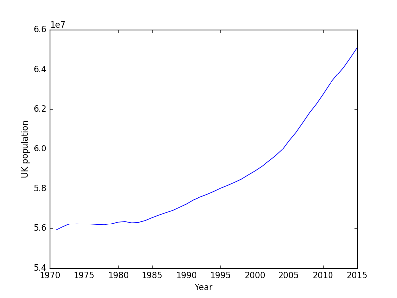
Passing simple data to the server: URL encoded arguments
Very simple data passing to the server is often done in the form of URL parameters.
Whenever you have seen a url that looks like, e.g.
https://www.google.co.uk/webhp?ie=UTF-8#q=python
(feel free to click on the link!) you are passing information to the server.
In this case the information is the form of two variables, ie=UTF-8 and
q=python. The first is presumably inforation about the encoding that my
browser requested, and the second is the query term I had asked for, in
this case from Google.
Simple URL arguments follow an initial question mark, ?, and are ampersand (&) separated key=value pairs.
Google uses a fragment identifier, which starts at the hash symbol #
for the actual query part of the request, q=python.
For such websites, passing data to the server is a relatively simple task of determining which query parameters the site takes, and then encoding your own.
For example if we create a list of search terms
terms = [
	"python image processing",
	"python web scraping",
	"python data analysis",
	"python graphical user interface",
	"python web applications",
	"python ploting",
	"python numerical analysis",
	"python generators",
]
we could generate valid search URLs using
baseurl = "https://www.google.co.uk/webhp?ie=UTF-8#q="
urls = [ baseurl + t.replace(" ", "+") for t in terms ]

for url in urls:
	# Perform request, parse the data, etc
Here we simply determined the “base” part of the URL and then added on the search terms, replacing the human readable spaces with the “+” seperators.
urllib also provides a function to perform this parameter encoding for us,
data = {'name' : 'Joe Bloggs', 'age': 42 }
url_values = urllib.parse.urlencode(data)
print(url_values)
generates
age=42&name=Joe+Bloggs
For complicated encodings, this is certainly better than manually generating the parameter string.
Making POST requests
So far we have been dealing with what are known as GET requests.
GET was the first method used by the HTTP protocol (i.e. the Web).
Nowadays there are several more methods that can be used:
- GET
- HEAD
- POST
- PUT
- DELETE
- TRACE
- OPTIONS
- CONNECT
- PATCH
Most of these are relatively technical methods; the POST method, hoewever, is in widespread usage as the standard mechanism to send data to the server.
POST requests are commonly associated with forms on web pages. Whenever a form is submitted, a POST request is made at a specific URL, which then elicits a response.
Many web-based resources use forms to retrieve data.
Luckily for us, making a POST request is relatively straight forward with Python; the tricky part is usually determining the POST parameters.
For example, to POST data to Exeter Universities phone directory (http://www.exeter.ac.uk/phone/) we could use
import urllib.request
import urllib.parse
url = "http://www.exeter.ac.uk/phone/results.php"
data = urllib.parse.urlencode({"page":"1", "fuzzy":"0", "search":"Jeremy Metz"}).encode("utf-8")
req = urllib.request.Request( url, data=data )
text = urllib.request.urlopen(req).read().decode("utf-8")
Alternatives to urllib
urllib comes with Python and is relatively straight forward to use.
There are however alternative libraries that achieve the same tasks, such
as request, which aims to be a simple alternative to urllib.
For full web crawling tasks, scrapy is a popular web spider/crawler library,
but is beyond the scope of this section.
Dealing with Javascript rendered objects
Many modern websites use Javascript to generate generate content dynamically.
This makes things trickier when we try to scrape data from such pages, as the raw page text doesn’t contain the data we want!
Ultimately, we will need to run the Javascript to generate the data we want, and there are several options for doing so, including
- Selenium : A full web automation and testing framework
- ghost.py : webkit client
- dryscrape : A light-weight webikit client
- Build your own! : The PyQt5 library includes a web renderer!
Webkit, mentioned above, is the layout engine component used in many modern browsers like Safari, Google Chrome, and Opera (Firefox, on the other hand uses an equivalent engine called Gecko).
As an example, the site http://pycoders.com/archive/ contains a javascript generated list of archives.
Using PyQt5 we can pull this list using
import sys
from PyQt5.QtWidgets import QApplication
from PyQt5.QtCore import QUrl
from PyQt5.QtWebKitWidgets import QWebPage
from lxml import html

#Take this class for granted.Just use result of rendering.
class Render(QWebPage):
  def __init__(self, url):
    self.app = QApplication(sys.argv)
    QWebPage.__init__(self)
    self.loadFinished.connect(self._loadFinished)
    self.mainFrame().load(QUrl(url))
    self.app.exec_()

  def _loadFinished(self, result):
    self.frame = self.mainFrame()
    self.app.quit()

url = 'http://pycoders.com/archive/'
r = Render(url)
result = r.frame.toHtml()
htmltree = html.fromstring(result)
archive_links = htmltree.xpath('//div[2]/div[2]/div/div[@class="campaign"]/a/@href')
print(archive_links)