These notes are intended as an introduction to effective use of ImageJ, a mature image-processing platform created by the National Institute of Health (NIH).

There are many excellent ImageJ tutorials and resources available online. Notable examples include:

1. The original ImageJ site tutorials and examples: http://rsbweb.nih.gov/ij/docs/index.html
2. Newer ImageJ site tutorials: https://imagej.net/Category:Tutorials
3. EMBL/CMCI ImageJ resources (inc. textbook): http://cmci.embl.de/documents/ijcourses
4. CNRS MRI ImageJ workshop: http://dev.mri.cnrs.fr/wiki/imagej-workshop
5. Goettingen Astrophysics ImageJ tutorial/book: http://www.astro.physik.uni-goettingen.de/~hessman/ImageJ/Book/
6. The new ImageJ website http://imagej.net/Introduction

Whilst having been initiated for the medical and biological sciences, ImageJ, because of it’s extensible nature and large variety of plugins is now used in many disciplines requiring image processing.

A note about these notes!

These notes are not intended to be a comprehensive guide to all ImageJ functions and techniques; there are already many excellent online tutorials (some of which are listed above).

Rather than rehashing and rephrasing the contents of these other resources, the point of this workshop is to provide an environment for you to practice using ImageJ, with demonstrators at hand to help when you need it.

Working on your own data

A core component of this workshop is the idea that you would be able to practice what you’ve learned with help at hand.

During each session, after you have completed the exercises scheduled for that session you are invited to work on your own data on tasks relevant to your research. We will be at hand to help you out when you get stuck!

Printing the notes

For both environmental reasons and to ensure that you have the most up-to-date version, we recommend that you work from the online version of these notes.

A printable, single page version of these notes is available here.

Errata

Please email any typos, mistakes, broken links or other suggestions to j.metz@exeter.ac.uk.

Installing on your own machine

If you want to use imagej on your own computer I would recommend using Fiji which can be downloaded from

http://fiji.sc/Fiji

Fiji is ImageJ with additional functionality and bundled plugins.

Alternatively standard ImageJ can be downloaded from

https://imagej.net/Downloads

Starting ImageJ

As ImageJ is a Java program, it is relatively “portable” which means it can be run without being installed in the traditional way.

In general, you can always start ImageJ by navigating to the ImageJ folder and running the approprate executable. Executables are included for all major architectures and for 32 and 64bit machines.

If ImageJ has been installed as a system wide application it may be started via the start menu.

For example, on the Hatherly B12 machines, ImageJ may be started by clicking on the Start button and navigating to:

All Programs > Local Applications > College of Life Sciences > Biosciences

and select ImageJ.

Alternatively, or if ImageJ is not listed at that location, after pressing the Start button, type “imagej” into the search field and select imagej from the search results.

Starting Fiji instead

Fiji (Is Just Imagej) is a distribution of ImageJ that includes many of the most common and powerful additional plugins.

You will probably end up finding that it’s easier to use Fiji than installing the same plugins to ImageJ yourself!

Fiji may be located at

C:\Users\Public\Desktop\Fiji\Fiji.app

the executable to double click is (still) called ImageJ-win64.exe.

If Fiji is not at that location, it’s easiest to stick with the installed version of ImageJ for this workshop.

The main Toolbar

The core functionality in ImageJ is accessible via the menu bar shown below.

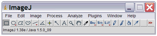
In the rest of this text, the notation

File > Open

indicates selecting first the “File” menu and then the “Open” Sub-menu/command.

Loading data

File > Open or File > Import (depending on data type).

Open is generally used for 2D data sets (images) and Import for 3D data sets, as it allows opening image sequences, multi-layer tiffs, and films (avis).

TIP: Drag and Drop image loading

For many image types you can also drag and drop the image from the file explorer onto the ImageJ toolbar

Exercise 1.1

Download the Cell_Colony.jpg sample image from https://imagej.net/images/.

After saving it on your desktop, open the image in ImageJ.

Additional: Also download the confocal stack files and the ct.dcm files to familiarise yourself with loading various image file formats.

Inspecting data

Before we move on to manipulating the image in any way, it’s sometimes useful to start out by examining the image.

There are several tools to help us get to know the data in imagej;

• image > show info gives use information like width, height, bit-depth, and scale (if set)
• hovering over the image with the mouse reveals the intensity that pixel location (displayed in the main toolbar’s status area)
• Use the line-selection tool to measure distances (see ROI section below)

Now that we’ve loaded some sample data and looked at it a bit, let’s take a step back and think about what that image is.

Similarity to other forms of measurements

If we were to use a thermometer to measure the temperature of a solution, or an electrode attached to a ammeter to measure a time-varying current, (such as for a patch-clamp experiment), we know that these measured quantities need to be recorded appropriately and subsequently analysed.

However, when dealing with images, our scientific approach is sometimes forgotten, and we treat images differently, not being careful about data format issues like bit-depth or lossless compression.

Human vision: the gold standard?

When it comes to “analysing” images, this is often left to “by-eye” classification, counting, etc.

While it’s true that our eyes and visual systems are fantastic at pattern recognition and classification, to the extent that in many cases they’re used as the ground-truth when evaluating image processing pipelines, unfortunately they’re not very good scientifically speaking.

This stems mainly from the fact that human perception is subjective, differing both between people and also between the same person at different times.

In addition, we’re not able to be very accurate when quantifying things by eye, such as brightness, size etc.

Pixels pixels everywhere

Before we move onto the more systematic and objective ways that computational image processing techniques (via in this case ImageJ) lets us analyse images, let us quickly recap what an image is.

Imaging aparatus

Most modern optical imaging aparatus consists of two main components; some form of focussing setup (e.g. lenses and mirrors), and the final detector that converts the optical signal (photons) into an electrical signal which will be stored.

The optical components and focussing stage determines for the most part the scale of the scene being imaged, and ranges from very large far away structures (telescope), through to medium to close range, everyday size objects (standard cameras), and finally down to resolving sub-cellular structures or even individual proteins (optical microscopes).

Once the optical signal has traversed the optical setup it is registered. When these systems were first invented, the only available registration medium was the eye (followed by drawing what was seen). Since then, photographic film has long been the standard for capturing images, until relatively recently, when digital image recording devices were introduced. Conceptually, these consist of a grid of individual detection units (currently CMOS and CCD are the most common types of sensor arrays).
Each detection unit converts the intensity of light into an electrical signal and the whole array of these signals is then encoded into an image format for storage.

There are many other types of setups which also produce images but don’t use light (photons), such as scanning electron microscopes, atomic force microscopes, ultrasound scanners to name a few. The image processing techniques available through ImageJ work equally well on these types of images also.

An image as an array

For many of these set-ups the images will consist of a grid of pixels. The grid has a width and height, which we will denote W and H, such that the grid can be represented by a WxH matrix/array.

[Image Source]

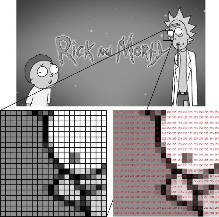
TIP: Pixel inspection tool

ImageJ comes with a “Pixel Inspector” plugin accessible via the toolbar:

• Click the >> symbol
• Select “Pixel inspector”
• Click and drag mouse over image to inspect pixel values.

Colours and grays

Most images that we’re used to from everyday life are in the form of colour images.

Usually this is stored using RGB (Red-Green-Blue) colour-space, which means that at each location in the image, three values are needed - the amount of red, the amount of blue, and the amount of green.

In this case, the image can be represented as having 3 dimensions, and being of size W x H x 3.

If we convert the colour image to grayscale, we combine the RGB channel information into a single quantity (usually a weighted sum of the R, G, and B channels).
This produces a single amount of gray at each location, and the image matrix returns to being two dimensional.

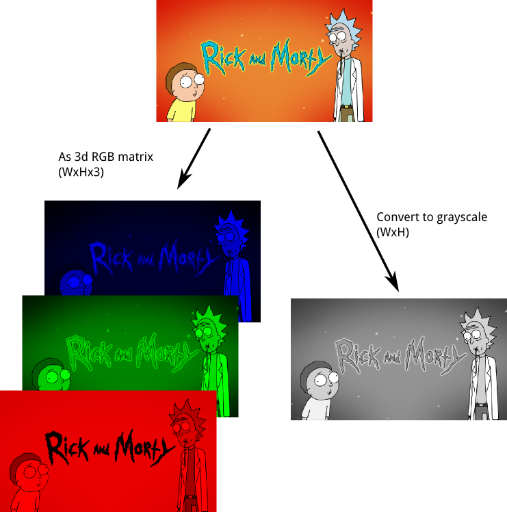
Image formats

Now we’ve covered how simple images come as grayscale (2d) or colour with where each pixel has 3 colour values, how about the file format that we use to store that imaging data to disk?

You’ll probably be familiar with some of the common image formats such as JPG/JPEG, PNG, and TIFF.

There is however a crucial difference between the way a format like JPG saves data and how PNG saves data. That difference is down to how the compression algorithms work, as both generally use compression to try and reduce the amount of space needed to store the image information.

JPG uses lossy compression, while PNG uses lossless compression.

Put another way, if pixels were documents, then essentially PNG is similar to a standard ZIP archive, while JPG is like an aggressive archive format which decides which documents are worth keeping, and throws away the rest!

You may have found that JPG files are generally smaller than PNG - now you know why. The “loss of pixels” corresponds to the “compression artifacts” that you may have noticed (especially on more heavily compressesed JPGs) which often look block-like.

TIFF, and in particular, OME-TIFFs are a feature-rich format that allow saving multiple stacks, as well as a wealth of meta-data with your image data. Note however that TIFF does allow for JPG compression, so make sure you never select this when saving data as TIFFs. Also, as OME-TIFF is relatively new, it’s not very widely supported.

PNG on the other hand is a relatively simple format that supports upto 16 bits per channel and upto 4 channels (RGB which we talked about above, and an “alpha” channel which holds transparency information, aka RGBA). There are many additional, proprietary formats - such as Zeiss ZVI, and Leica’s LSM formats.

I would generally recommend avoiding proprietary formats / converting to a more open format such as TIFF (or PNG if appropriate).

Bitdepth

The bitdepth or bits-per-pixel (bpp) of an image format refers to the number of bits that are used to store each pixel value. The lowest common bit-depth is 8 bpp, which means that 8 bits are used to store each pixel value. As it is only possible to store 256 (2^8) distinct values with 8 bits, such images usually range between 0 and 255 and will only contain integers.

Scientific data often comes with the option to save at higher bit-depths (usually up to 16 or 32 in some cases) which allows for 65536 values to be stored (2^16) - providing a much wider range of intensities, and therefore detail. Be aware that storing grayscale data using an 24-bit RGBA format actually only
stores 8 bits per channel - the colour channels will all simply be replicating the same data!

Now that we’ve had a quick introduction to what an image is, and available image formats, let’s get started with ImageJ!

TIP: Making up for ImageJ’s shortcomings

While being a generally poerful and useful framework, ImageJ has some quirks that require workarounds.

To save you running into these at a later stage, here are two common workflows:

undo don’t undo

ImageJ’s undo functionality is a little unreliable - some operations undo and others don’t! To work-around this, use duplicates of images (ctrl-shift-D) to keep regular, snapshots of your processing work.

Regions of Interest

Similarly to the undo, the ROI functionality is a little inconsistent - some functions will operate only inside an ROI while others will still operate on the whole image.

A simple work-around is to use the ROI to crop out your region of interest.

Cleaning data

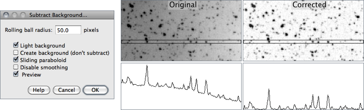
Often data will contain a bright (and sometimes variable) background. ImageJ implements a “rolling ball” filter to subtract this background;

Process > Subtract Background

The choice of ball radius should be larger than the maximum object radius that isn’t background. The action of the filter can be likened to rolling a sphere of given radius “under” the image data - the background that is subtracted is the top-most reach of the sphere.

ROIs (Regions of Interest)

Simple ROIs can be created by using the first few (left-most) icons on the standard ImageJ toolbar, namely the area selection tools,

Once created, an ROI can be used to restrict the region over which subsequent processing and analysis are applied.

Complicated composite ROIs can also be generated and saved by using the ROI manager which can be accessed via

Edit > Selection > Add to Manager [Ctrl + t]

Exercise 1.2

Open the modified cell colony images available from

• Cell_Colony1.jpg
• Cell_Colony2.jpg

and select your choice of rectangular region of the image. Apply the background subtraction function to the region - you will find that this is not the default mode of operation for subtract background - try and figure out how to do this. Experiment with the light background setting and confirm that it produces the result that you would expect.

Thresholding

Binary masks, which are similar to ROIs, can also be generated by performing segmentation on the image. One of the simplest segmentation operations is thresholding. Simple thresholding marks all pixels with values less than the threshold as off or 0, and all pixels with values equal to or above the threshold as on or 1.

To apply a simple threshold to the image use

Image > Adjust > Threshold [Ctrl + Shift + t]

This opens a thresholding dialog

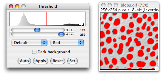
which allows us to see which regions will be included.

Statistics

Image statistics, as well as advanced statistics and measurements can be accessed via the Analyse menu.

For example, simply running Measure on an open image returns the Area, Mean, Min and Max of the whole image.

Usually ROIs are first generated, either manually, or by using first generating a binary image. This can be achieved by simple thresholding as outlined above or a more advanced technique.

Once the image is binarized, use Measure > Analyze particles to measure each each binary region.

These can also be turned into individual ROIs by selecting “Add to manager”, and then later used on, for example, the original image.

Exercise 1.3

Using the Cell_Colony1.jpg file as input, first subtract the background (remember to use the dark on light option!) and then measure particle sizes in a polygonal ROI.

Small object removal

There are multiple approaches to removing small objects, which may correspond to noise, dust, or other unwanted imaging phenomena in imagej. These include

• Process > Noise > Despeckle
• Process > Noise > Remove outliers
• Process > Binary > Open

The most basic of these is (morphological) opening which, is defined as the dilation of the erosion of a binary image.

Exercise 1.4

Repeat exercise 1.3 - but this time before measuring the objects, experiment with the three techniques for small object removal to familiarize yourself with the differences between them.

Advanced thresholding: Otsu and friends

We performed simple thresholding operations in the last section, which involved manually selecting a value at which to separate objects from background.

Less subjective, automated methods for background estimation, or segmentation, also exist.

These include

• IsoData algorithm (the default when using imagej’s Threshold)
• Otsu’s method
• Huang
• Intermode
• Li
• MaxEntropy
• … and several others!

They each have strengths and weaknesses, which depend on the underlying assumptions made.

For example, I routinely use a technique called Median Absolute Deviation (MAD) to estimate the background noise level and variance, and select as signal anything that is ~ 3 variances greater than the background level as it has a very clear assumption about the background level (namely that it is normally distributed noise).

I recommend that you experiment with the various segmentation techniques to find the one that best suits your application.

Exercise 2.1

Repeat the thresholding from exercise 1.3, but experiment with the various automatic thresholding techniques instead of manually selecting the level.

Advanced segmentation: distance transform and watershed

We saw in the simple thresholding that bright areas that touch generally get counted as part of the same region. In some cases this is not desirable as for example we could have multiple cells that are close together.

One technique to overcome this clumping is to use what is known as the watershed transform.

A detailed explanation of the watershed transform can be found here and on wikipedia.

While in some instances applying the watershed transform directly can yield good results, in general there is too much noise in an image to get good segmentation this way. Therefore a common approach is to apply a sequence of operations,

1. Threshold image to create binary image
2. Perform a distance transform (~“distance from each 1 pixel to the nearest 0 pixel”)
3. Perform watershed on distance transform of image
4. Apply the boundaries from the watershed result to the binary image.

ImageJ contains a function which combined steps 2-4, which is calls watershed under

Process > Binary > Watershed

For example, after converting the blobs sample image to binary we have

Then calling watershed gives

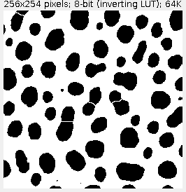
Additional details on the distance transform can be found here .

Exercise 2.2

Repeat exercise 1.3, and then perform the same operation, but using the watershed operation before the measurement.

You should notice that there are more objects, some having smaller areas than before. The total area should remain unchanged as we should only have split some touching objects.

Scale space filtering

Scale-space filtering is an advanced filtering technique which enables the extraction of object sizes as well as positions.

The idea is to blur an image at a range of scales, and by combining these scales in the right way 1, one finds that peaks in the resulting nD + 1 (e.g. 2D + 1 = 3D for images) data gives both object positions, x,y,(z..) as well as approximate sizes.

Details

The main operations involved are Gaussian filtering, and taking image derivatives. The motivation for this is that, object peaks correspond to minima in the second derivative, i.e. the change in the curvature, of the smoothed image data.

For example if we were attempting to get positions and sizes of cells, we wouldn’t want to get peaks corresponding to vesicles and other objects that cause the cell image to have small-scale peaks. Therefore we first blur the image over a range of scales such that the minimum scale is smaller than any cell size but larger than any subcellular details, and the maximum scale is larger than any cell size, but smaller than clusters of cells.

This ensures that the peaks in the resulting scale-space representation correspond to cells, and not to subcellular structures or groups of clustered cells.

ImageJ doesn’t contain a scale-space plugin, but the basic operations which allow us to approximate the action of a single scale selection are as follows 2:

1. Gaussian filter copy 1 at scale s1
2. Gaussian filter copy 2 at scale 1.6*s1
3. Process > Image Calculator
4. Select subtract for operation and subtract result 1. from result 2.

The resulting image has been scale-space filtered at scale 1.3 x s1.

We’ll find a more useful way of implementing this when we come to macros.

More details about scale-space blob detection can be found here.

Going beyond basic ImageJ functionality : Using plugins

Plugins add to the core ImageJ functionality and provide many of the more specialized functions useful for more advanced image processing tasks.

Installation

The NIH maintain a repository of hundreds of ImageJ plugins here: http://rsbweb.nih.gov/ij/plugins/.

Installation of plugins is straightforward and can usually be achieved by saving the plugin into the ‘plugin’ folder in the ImageJ directory.

Useful plugins and ImageJ distributions

Below is a short list of very useful plugins.

Bioformats

The bioformats plugin contains import functionality for a large range (apparently numbering over 100) of proprietary biological data filetypes.

It also supports 4-d and 5-d data sets, i.e. xyztc, meaning three spatial dimensions, time, and channel information.

Colocalization

The colocalization functionality in ImageJ is not actively maintained, and apparently buggy [http://fiji.sc/Colocalization_Analysis]. Instead Coloc_2 or JACoP imageJ plugin provide extensive colocalization tools, such as

“…pixel intensity correlation over space methods of Pearson, Manders, Costes, Li and more, for scatterplots, analysis, automatic thresholding and statistical significance testing.”.

3D Viewer

This plugin enables 3D data visualization from within ImageJ including ortho-slices, isosurfaces, and addition of simple 3d primitive shapes (e.g. spheres).

See http://rsbweb.nih.gov/ij/plugins/3d-viewer/

Fiji

Fiji is not a plugin, but a redistribution of ImageJ (as the name FIJI: Fiji is just imagej implies!) with many useful plugins included. This includes the bio-formats plugins for reading a large variety of microscopy files, as well as a large range of filters and analysis plugins.

BoneJ

BoneJ http://bonej.org/ is a collection of plugins developed for tubular geometry and whole bone shape analysis.

Exercise 2.3

Note

If you are already using FIJI, you should already have the following plugins installed - in which case only practice using these plugins.

Download and install the bioformats and 3d Viewer plugins mentioned above. Use them to visualize a 3d data set of your choice, adding an isosurface representation that makes the structures in the data set visible (Note that you may need to apply some background filtering to achieve good isosurface segmentation!).

If you’re feeling adventerous, also try downloading and installing any additional plugins that might be interesting for your work.

Memory usage

When working with larger datasets, you will need to consider the memory used to store the data in memory (RAM) - including intermediate processing.

For most standard images this is not an issue, but when working with large three or four dimensional datasets (e.g. time-series or z-stacks with multiple channels), you will likely run into memory issues.

There are two common strategies for dealing with memory issues when using large datasets

• Increase the amount of memory available to ImageJ (see below)
• Chunk the data

ImageJ is configured to use a relatively small amount of memory (usually 128-640 MB). If this is not enough to process your images, you will get a memory error. To increase the amount of memory available, go to Edit > Options > memory and increase the amount available. You will want to keep this less than 75% of your available system memory. If you are using a 32 bit OS (All older windows installations except XP64 and Vista64), you must set it to less than 1700 mb, or ImageJ will crash when launched.

Note

You will probably not be able to change the amount of memory ImageJ uses on the computing suite computers. However, navigate to the appropriate menu option to familiarize yourself with the location of this very useful option!

Chunking data is only applicable in some scenarios, and a basic form of this is available through using ImageJ’s virtual stack loading option.

In general, chunking means to work on small chunks of data at a time, thereby only loading small amounts of data into memory at a time while leaving the majority of the data on disk. For stacks, this is straight-forward to understand in terms of loading a frame or slice at a time. Similar approaches include tiling data, and multi-resolution loading, but go beyond the capabilities of standard ImageJ.

Imagej has a macro system to allow the user to rapidly repeat a set of commands without having to execute each one individually.

For example, you may want to automate counting “blob”-like objects in images, which requires that you blur the image, then find maxima, and finally count the number of peaks.

Instead of running all three operations on each input image, the easiest way to create a macro is to let imagej record it when you perform the sequence of actions once.

There is a separate course on ImageJ Macros, but in the following section we’ll look at creating macros via the User Interface.

Even without looking at the macro code at all, Recording Macros is a good way of keeping track of the processing that you apply to data.

Recording macros

First open an image that you will process. This operation will not be included in the macro at this point.

Next press Plugins > Macros... > Record ... to open up the macro recording dialog (“Recorder”).

The recording has begun; any subsequent operations will appear in the Recorder dialog.

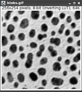
As an example after having opened Blobs from the samples (Hint: Use Ctrl+Shift+B), start the recorder.

Next perform the following operations:

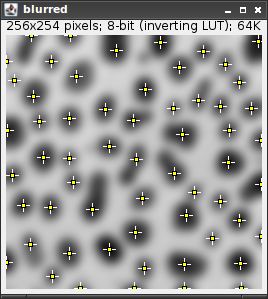
1. Image > Duplicate ...
2. Set the title to “Blurred”
3. Process > Filters > Gaussian Blur...
4. Enter sigma = 5
5. Press OK
6. Process > Find Maxima...
7. Check “Light Background”
8. Press OK
9. Analyze > Measure

The Results window will show various measurements for the detected peaks (there should be 59!).

The Recorder window should show

run("Duplicate...", "title=blurred");

run("Gaussian Blur...", "sigma=5");

run("Find Maxima...", "noise=10 output=[Point Selection] light");

run("Measure");

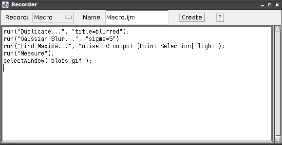
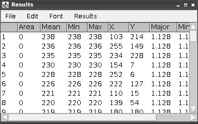
which summarizes the operations we performed.

This macro can be saved using the Create button to save the macro with the name specified in the “Name” field. This will open a save file dialog. Confirm that the filename is one that makes sense to you and a usual location is the imagej/Macros folder, then go ahead and save the Macro.

The macro can be applied on any loaded image by calling

Plugins > Macro > Run...

and finding and selecting the macro we just saved.

Exercise 2.4

Use the above approach to apply the Gaussian filter to the blobs data set over a short range of blur radii. At each scale, find the peak locations.

run("Gaussian Blur...", "sigma=1");
run("Find Maxima...", "noise=10 output=[Point Selection] light");
run("Measure");
run("Gaussian Blur...", "sigma=2");
run("Find Maxima...", "noise=10 output=[Point Selection] light");
run("Measure");
run("Gaussian Blur...", "sigma=3");
run("Find Maxima...", "noise=10 output=[Point Selection] light");
run("Measure");
run("Gaussian Blur...", "sigma=4");
run("Find Maxima...", "noise=10 output=[Point Selection] light");
run("Measure");

for(scale=1; scale <= 4; scale = scale + 1){
    run("Gaussian Blur...", "sigma="+scale);
    run("Find Maxima...", "noise=10 output=[Point Selection] light");
    run("Measure");
}

Batch processing

Working with large data sets

In the previous section, we didn’t automate opening the file with the recorder because otherwise the macro would have recorded:

run("Blobs (25K)");

which is only relevant for that data set. Often we are working with many data sets, or a data set with many frames. In such cases, hard coding the filename, or slice number, is not useful as the macro would run the operations on the same file/frame each time it is run.

Probably the simplest option is to use imagej’s

Process > Batch > Macro...

functionality.

This allows one to select a source folder that contains a set of input files, and a source folder to store results.

In addition the edit box allows selection of the operations that are to be performed.

The same functionality for a loaded stack can be obtained by using

Process > Batch > Virtual Stack...

Exercise 2.5

Download a stack composed of multiple images from the ImageJ website such as some of the images in

http://imagej.nih.gov/ij/images/pet-series/

to a new folder (called, e.g. “Stack files”).

Next start the batch processor, set the input directory to the Location you downloaded the stack files to, and select a macro to perform on the series. Create a new directory called “output” and use that as the output directory for the batch operation.

Summary

Hopefully the hours that you’ve spent in the workshop have been useful in getting started with ImageJ.

As pointed out at the beginning of the workshop, the aim was not to bombard you with a list of function after function of all of the filters, analyses, and pipelines that ImageJ has to offer, but rather to provide an environment for you to explore ImageJ at your own pace, with demonstrators at hand to help out when needed.

Nonetheless, you should now be relatively comformtable with the following simple operations and concepts

• Loading a variety of images
• Inspecting image data, and understanding that a digital image is essentially a grid of numbers
• Simple image operations, such as background removal using a rolling ball filter
• Be aware that there is much more functionality available via the extensive list of plugins
• Understand why recording macros is a good idea, and how to record a macro

Next steps

Now that you are familiar with the basics of ImageJ, the best way to improve and learn more is to practice!

In addition there is one further session on ImageJ macro editing where I will introduce how to edit the recorded macros to become more powerful, as well as showing how to write a macro from scratch!

Note

Some of the concepts related to editing macros overlap with general programming concepts; be prepared for a relatively steep learning curve if you are entirely unfamiliar with all programming concepts, as we won’t have time to cover these in the single workshop session!

Optional Exercises

As emphasised throughout the workshop, ideally you will have brought your own data to process, or have managed to find similar data from other sources (e.g. colleagues, online).

This is so that the techniques and skills you learn are those that are most relevant to your work.

However, if you were not able or for some other reason prefer not to work on such data, I have provided a handful of additional exercises below to practice your image processing skills on.

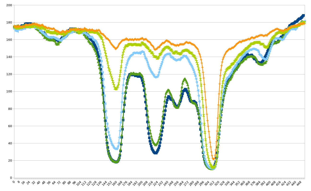
a) Quantifying an electrophoresis gel image

Download the sample data from

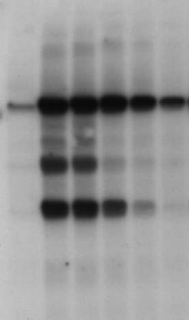
Typically such images are used as evidence of the presence or absence of macromolecules and their fragments (more info here for example: https://en.wikipedia.org/wiki/Gel_electrophoresis ).

Your task is to try and quantify the data in this image (e.g. quantitatively how dark is each band?).

Hint

One approach to this might be to try and replace the 2d image with a sequence of 1d data (as each “lane” corresponds to roughly 1d information). In that case you should, as an intermediate output generate a plot similar to (but hopefully better than!) the following

]

If you have other ideas for how to tackle this problem, please feel free to experiment and compare!

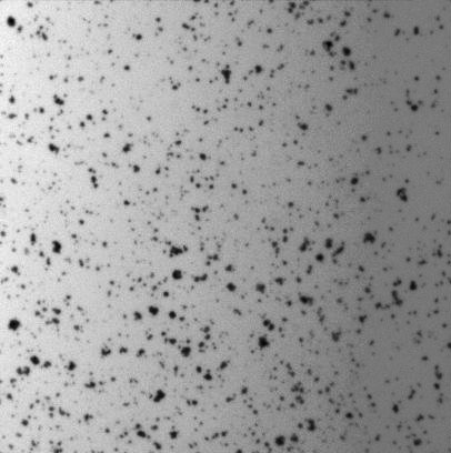
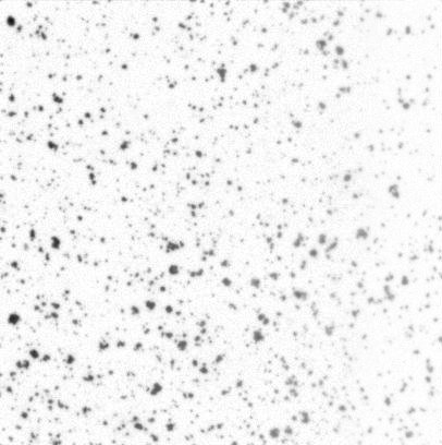
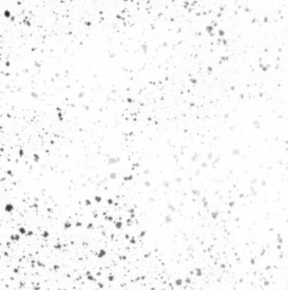
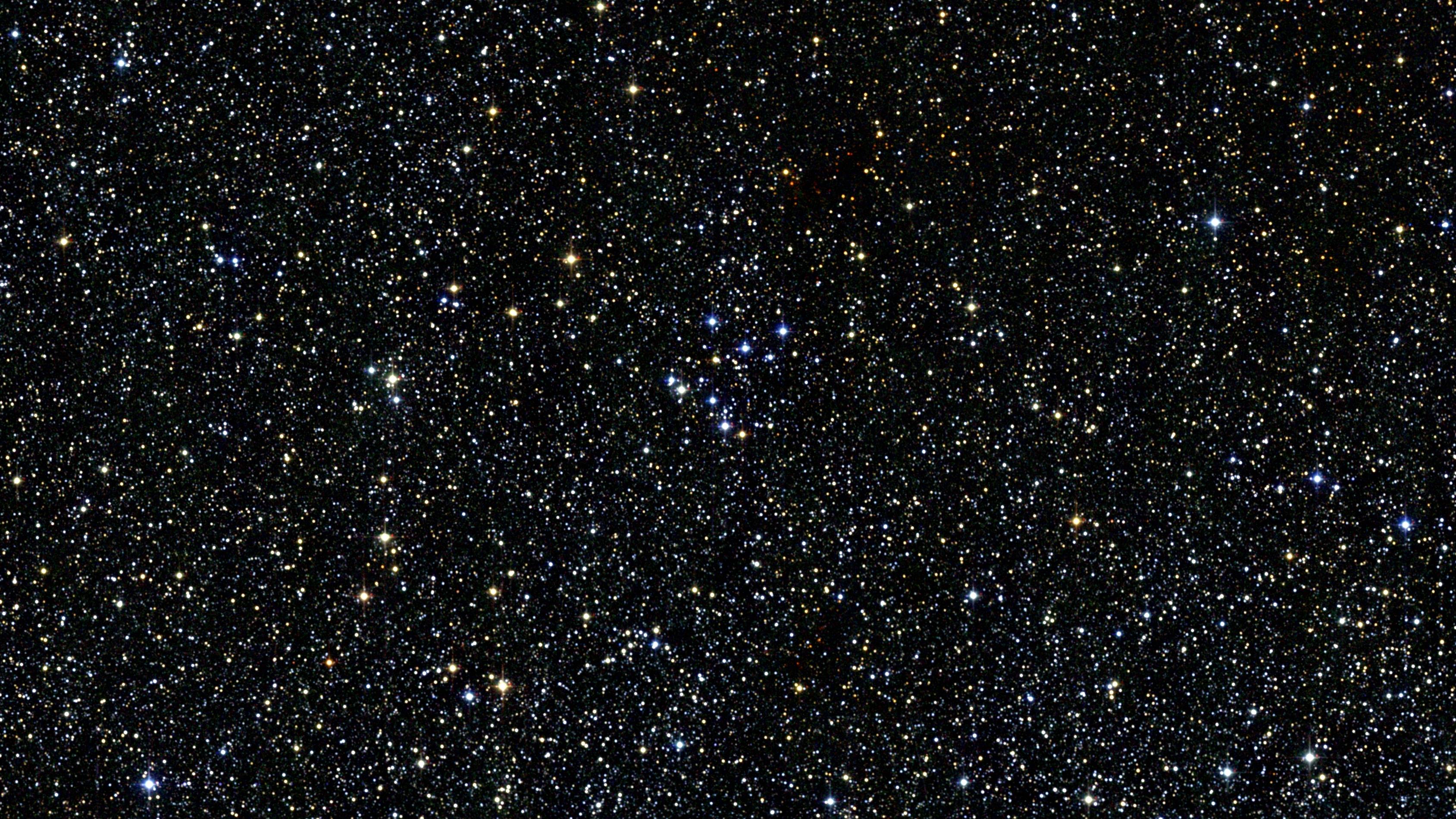
b) Counting and analysing stars

Download the image from here.

Try and come up with a processing workflow that let’s you

• Count the number of stars
• Compute the size distribution
• Compyte the intensity distribution (mean intensity)
• Find out if size correlates with intensity

Note

Some of this is beyond the scope of ImageJ and you will need to use e.g. Excel to generate the corrlation
analysis.

This exercise, to some extents, shows us some of the limitations of ImageJ, compared with a framework with larger scope, i.e. which could also be used to perform these analyses, such as Matlab or Python.

More exercises?

If you need more exercises please ask a demonstrator to help you determine which types of data might be best for you, especially with regards to being similar to the type of data you are intending to analyse.